Titanic data visualiztion practice in R

Titanic dataset Visualization (from Kaggle)

• The original source is here below

  [https://www.kaggle.com/romabash/titanic-data-visualization]

• Download titanic.csv

Import required packages and data

# Load packages and Data
library(readr) # Reading in data
library(tidyverse)

── Attaching core tidyverse packages ──────────────────────── tidyverse 2.0.0 ──
✔ dplyr     1.1.3     ✔ purrr     1.0.2
✔ forcats   1.0.0     ✔ stringr   1.5.0
✔ ggplot2   3.4.4     ✔ tibble    3.2.1
✔ lubridate 1.9.3     ✔ tidyr     1.3.0
── Conflicts ────────────────────────────────────────── tidyverse_conflicts() ──
✖ dplyr::filter() masks stats::filter()
✖ dplyr::lag()    masks stats::lag()
ℹ Use the conflicted package (<http://conflicted.r-lib.org/>) to force all conflicts to become errors

library(ggthemes) # Data visualization
library(RColorBrewer) # Data visualization
titanic <- read_csv("data/titanic.csv")

Rows: 891 Columns: 12
── Column specification ────────────────────────────────────────────────────────
Delimiter: ","
chr (5): Name, Sex, Ticket, Cabin, Embarked
dbl (7): PassengerId, Survived, Pclass, Age, SibSp, Parch, Fare

ℹ Use `spec()` to retrieve the full column specification for this data.
ℹ Specify the column types or set `show_col_types = FALSE` to quiet this message.

nrow(titanic)

[1] 891

head(titanic)

# A tibble: 6 × 12
  PassengerId Survived Pclass Name    Sex     Age SibSp Parch Ticket  Fare Cabin
        <dbl>    <dbl>  <dbl> <chr>   <chr> <dbl> <dbl> <dbl> <chr>  <dbl> <chr>
1           1        0      3 Braund… male     22     1     0 A/5 2…  7.25 <NA> 
2           2        1      1 Cuming… fema…    38     1     0 PC 17… 71.3  C85  
3           3        1      3 Heikki… fema…    26     0     0 STON/…  7.92 <NA> 
4           4        1      1 Futrel… fema…    35     1     0 113803 53.1  C123 
5           5        0      3 Allen,… male     35     0     0 373450  8.05 <NA> 
6           6        0      3 Moran,… male     NA     0     0 330877  8.46 <NA> 
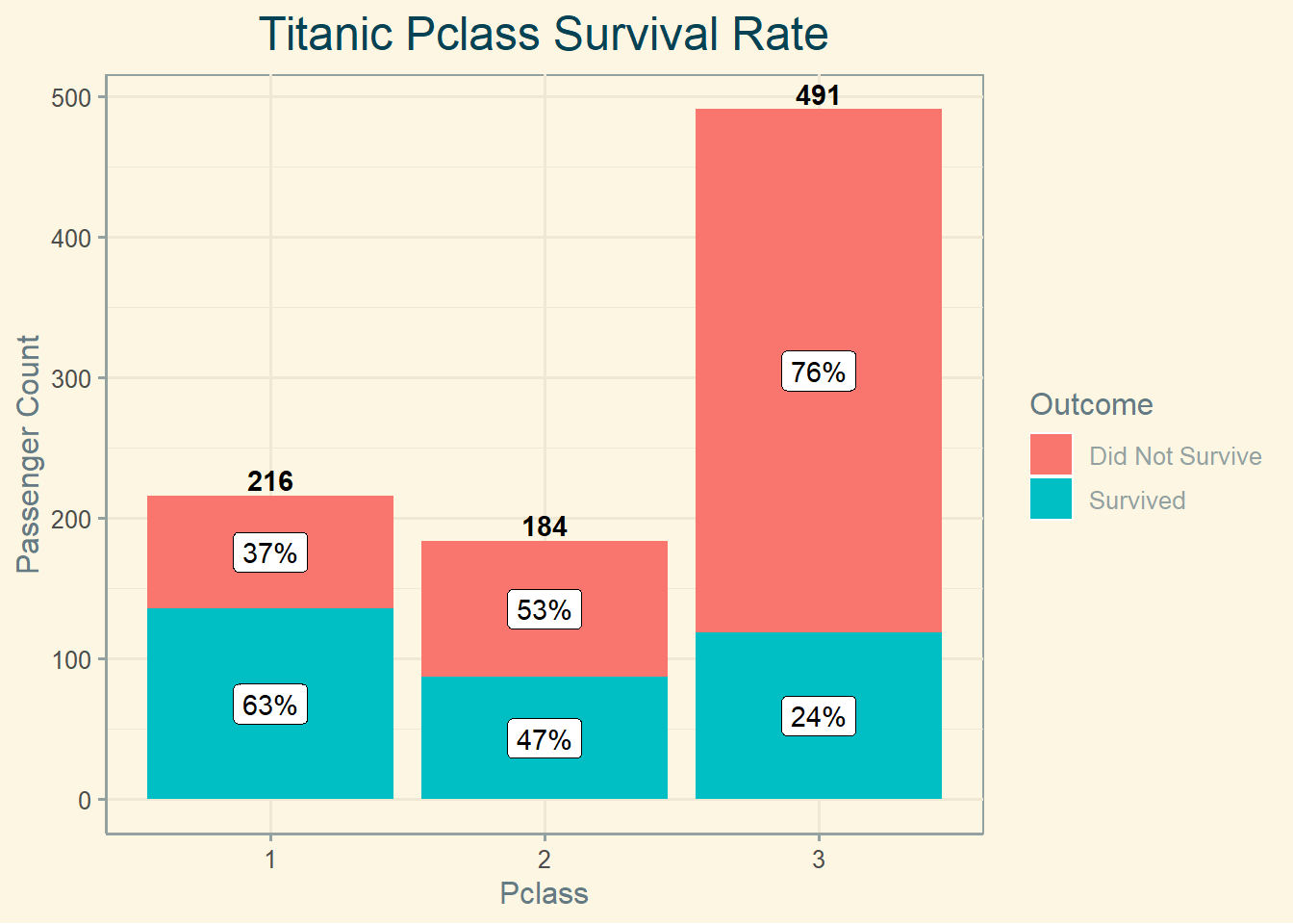
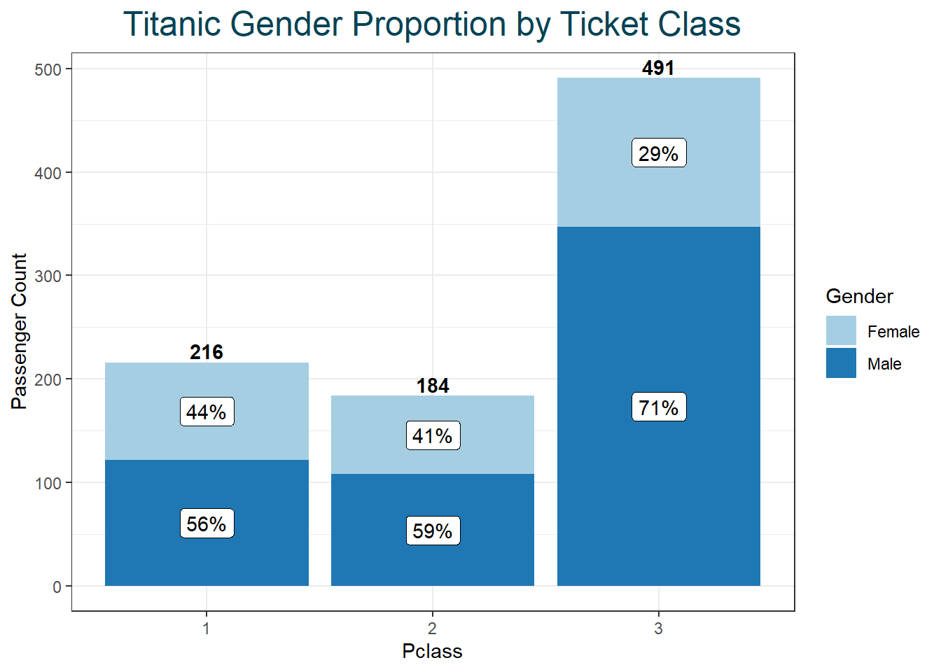
# ℹ 1 more variable: Embarked <chr>

table(titanic$Pclass)

  1   2   3 
216 184 491 

Pre-processing

# Convert Variable into Factors
# Convert Pclass, Survived and Sex Variables into Factors using the mutate function
# Keep Age numeric

str(titanic)

spc_tbl_ [891 × 12] (S3: spec_tbl_df/tbl_df/tbl/data.frame)
 $ PassengerId: num [1:891] 1 2 3 4 5 6 7 8 9 10 ...
 $ Survived   : num [1:891] 0 1 1 1 0 0 0 0 1 1 ...
 $ Pclass     : num [1:891] 3 1 3 1 3 3 1 3 3 2 ...
 $ Name       : chr [1:891] "Braund, Mr. Owen Harris" "Cumings, Mrs. John Bradley (Florence Briggs Thayer)" "Heikkinen, Miss. Laina" "Futrelle, Mrs. Jacques Heath (Lily May Peel)" ...
 $ Sex        : chr [1:891] "male" "female" "female" "female" ...
 $ Age        : num [1:891] 22 38 26 35 35 NA 54 2 27 14 ...
 $ SibSp      : num [1:891] 1 1 0 1 0 0 0 3 0 1 ...
 $ Parch      : num [1:891] 0 0 0 0 0 0 0 1 2 0 ...
 $ Ticket     : chr [1:891] "A/5 21171" "PC 17599" "STON/O2. 3101282" "113803" ...
 $ Fare       : num [1:891] 7.25 71.28 7.92 53.1 8.05 ...
 $ Cabin      : chr [1:891] NA "C85" NA "C123" ...
 $ Embarked   : chr [1:891] "S" "C" "S" "S" ...
 - attr(*, "spec")=
  .. cols(
  ..   PassengerId = col_double(),
  ..   Survived = col_double(),
  ..   Pclass = col_double(),
  ..   Name = col_character(),
  ..   Sex = col_character(),
  ..   Age = col_double(),
  ..   SibSp = col_double(),
  ..   Parch = col_double(),
  ..   Ticket = col_character(),
  ..   Fare = col_double(),
  ..   Cabin = col_character(),
  ..   Embarked = col_character()
  .. )
 - attr(*, "problems")=<externalptr> 

titanic <- titanic %>%
  mutate(Pclass = factor(Pclass), 
         Survived = factor(Survived), 
         Sex = factor(Sex))

titanic %>% glimpse

Rows: 891
Columns: 12
$ PassengerId <dbl> 1, 2, 3, 4, 5, 6, 7, 8, 9, 10, 11, 12, 13, 14, 15, 16, 17,…
$ Survived    <fct> 0, 1, 1, 1, 0, 0, 0, 0, 1, 1, 1, 1, 0, 0, 0, 1, 0, 1, 0, 1…
$ Pclass      <fct> 3, 1, 3, 1, 3, 3, 1, 3, 3, 2, 3, 1, 3, 3, 3, 2, 3, 2, 3, 3…
$ Name        <chr> "Braund, Mr. Owen Harris", "Cumings, Mrs. John Bradley (Fl…
$ Sex         <fct> male, female, female, female, male, male, male, male, fema…
$ Age         <dbl> 22, 38, 26, 35, 35, NA, 54, 2, 27, 14, 4, 58, 20, 39, 14, …
$ SibSp       <dbl> 1, 1, 0, 1, 0, 0, 0, 3, 0, 1, 1, 0, 0, 1, 0, 0, 4, 0, 1, 0…
$ Parch       <dbl> 0, 0, 0, 0, 0, 0, 0, 1, 2, 0, 1, 0, 0, 5, 0, 0, 1, 0, 0, 0…
$ Ticket      <chr> "A/5 21171", "PC 17599", "STON/O2. 3101282", "113803", "37…
$ Fare        <dbl> 7.2500, 71.2833, 7.9250, 53.1000, 8.0500, 8.4583, 51.8625,…
$ Cabin       <chr> NA, "C85", NA, "C123", NA, NA, "E46", NA, NA, NA, "G6", "C…
$ Embarked    <chr> "S", "C", "S", "S", "S", "Q", "S", "S", "S", "C", "S", "S"…

# Age has some missing values (NA). Missing values will be ignored for now

1. Look at the Total Survival Rate

#######################################
# 1. Look at the Total Survival Rate
# Use table function to look at the Survival rates
# Convert table to a tibble (similar to dataframe) to use later when plotting with ggplot2 to add text to the graph
# Use rename function to rename default Column names

str(table(titanic$Survived))

 'table' int [1:2(1d)] 549 342
 - attr(*, "dimnames")=List of 1
  ..$ : chr [1:2] "0" "1"

as.data.frame(table(titanic$Survived))

  Var1 Freq
1    0  549
2    1  342

survival <- table(titanic$Survived) %>%
  as.data.frame() %>%
  rename(Survived = Var1, Count = Freq)

survival

  Survived Count
1        0   549
2        1   342

titanic %>% 
  group_by(Survived) %>% 
  summarize(Count=n())

# A tibble: 2 × 2
  Survived Count
  <fct>    <int>
1 0          549
2 1          342

# Look at the Total Survival Rate Proportion
# Use prop.table to get the proportion

survival_ratio <- table(titanic$Survived) %>% prop.table %>% 
  as.data.frame() %>%
  rename(Survived = Var1, Percentage = Freq) %>%
  mutate(Percentage = round(Percentage, 2)*100)

survival_ratio

  Survived Percentage
1        0         62
2        1         38

# Plot the Total Survival Rate
# Using a barplot with theme_few theme from the ggthemes package
# Add some styling to the plot: Center the Title and color, Edit the Legends
# Use tibble of survival data in geom_text to add the Count to the plot
# Use tibble of survival data ratio in geom_label to add the Percentages to the bars



# survival_ratio %>% 
#   mutate(y=c(300, 200)) ->survival_ratio

survival %>% 
  mutate(lab=c("NS", "S"))-> survival

survival_ratio %>% 
  mutate(cordi=c(300, 190)) -> survival_ratio



titanic %>%
  ggplot() +
  geom_bar(aes(x = Survived, fill = Survived)) +
  geom_text(data = survival, 
            aes(x = Survived, y = Count, label = Count), 
            position = position_dodge(width=0.1),
            vjust=-0.25,
            fontface = "bold") +
  geom_label(data = survival_ratio, 
             aes(x = Survived, y = Percentage, label = paste0(Percentage, "%"), group = Survived), 
             position = position_stack(vjust = 5)) +
  theme_few() +
  theme(plot.title = element_text(hjust = 0.5, size=18, color = "#054354")) +
  ggtitle("Titanic Total Survival Rate") +
  scale_x_discrete(name= "Survival Rate", labels = c("Did Not Survive", "Survived")) +
  scale_y_continuous(name = "Passenger Count") +
  scale_fill_discrete(name = "Outcome", labels = c("Did Not Survive", "Survived"))

2. Look at Survival Rate by Gender

# Group the data by Sex using the group_by function
# Get the total Count of passengers in each gender group with summarise function

gender <- titanic %>%
  group_by(Sex) %>%
  summarise(Count = n())

table(titanic$Sex) %>% 
  as.data.frame %>% 
  rename(Sex=Var1,Count=Freq)

     Sex Count
1 female   314
2   male   577

gender

# A tibble: 2 × 2
  Sex    Count
  <fct>  <int>
1 female   314
2 male     577

# Look at the Gender Survival Rate Proportion
# Group by Sex and Survived to get the Count of survived by gender using summarise function
# Use mutate to add a new Percentage variable
gender_ratio <- titanic %>%
  group_by(Sex, Survived) %>%
  summarise(Count = n()) %>%
  mutate(Percentage = round(Count/sum(Count)*100))

`summarise()` has grouped output by 'Sex'. You can override using the `.groups`
argument.

gender_ratio

# A tibble: 4 × 4
# Groups:   Sex [2]
  Sex    Survived Count Percentage
  <fct>  <fct>    <int>      <dbl>
1 female 0           81         26
2 female 1          233         74
3 male   0          468         81
4 male   1          109         19

# Plot the Gender Survival Rate
# Using a barplot
# Represent Gender on the x-axis
# Use Color to represent Survival on the Plot
# Add the Count and Percentage using geom_text and geom_label respectively

titanic %>%
  ggplot() +
  geom_bar(aes(x = Sex, fill = Survived)) +
  geom_text(data = gender, 
            aes(x = Sex, y = Count, label = Count), 
            # position = position_dodge(width=0.9), 
            vjust=-0.25, 
            fontface = "bold") +
  geom_label(data = gender_ratio, 
             aes(x = Sex, y = Count, label = paste0(Percentage, "%"), group = Survived), 
             position = position_stack(vjust = 0.5)) +
  theme_few() +
  theme(plot.title = element_text(hjust = 0.5, size=18, color = "#054354")) +
  ggtitle("Titanic Gender Survival Rate") +
  scale_x_discrete(name= "Gender") +
  scale_y_continuous(name = "Passenger Count") +
  scale_fill_discrete(name = "Outcome", labels = c("Did Not Survive", "Survived"))

3. Look at Survival Rate by Ticket Class

# 3. Look at Survival Rate by Ticket Class
# Group the data by Pclass using the group_by function
# Get the total Count of passengers in each Pclass with summarise function

pclass <- titanic %>%
  group_by(Pclass) %>%
  summarise(Count = n())

pclass

# A tibble: 3 × 2
  Pclass Count
  <fct>  <int>
1 1        216
2 2        184
3 3        491

# Look at the Pclass Survival Rate Proportion
# Group by Pclass and Survived to get the Count of survived in each Pclass using summarise function
# Use mutate to add a new Percentage variable
pclass_ratio <- titanic %>%
  group_by(Pclass, Survived) %>%
  summarise(Count = n()) %>%
  mutate(Percentage = round(Count/sum(Count)*100))

`summarise()` has grouped output by 'Pclass'. You can override using the
`.groups` argument.

pclass_ratio

# A tibble: 6 × 4
# Groups:   Pclass [3]
  Pclass Survived Count Percentage
  <fct>  <fct>    <int>      <dbl>
1 1      0           80         37
2 1      1          136         63
3 2      0           97         53
4 2      1           87         47
5 3      0          372         76
6 3      1          119         24

# Plot the Gender Survival Rate
# Using a barplot using black and white theme theme_bw from ggplot2
# Represent Pclass on the x-axis
# Use Color to represent Survival on the Plot
# Add the Count and Percentage using geom_text and geom_label respectively

# pclass %>% 
#   mutate(lab=c("First", "Business", "Economy"))->pclass



titanic %>%
  ggplot() +
  geom_bar(aes(x = Pclass, fill = Survived)) +
  geom_text(data = pclass, 
            aes(x = Pclass, y = Count, label = Count), 
            position = position_dodge(width=0.9), 
            vjust=-0.25, 
            fontface = "bold") +
  geom_label(data = pclass_ratio, 
             aes(x = Pclass, y = Count, label = paste0(Percentage, "%"), group = Survived), 
             position = position_stack(vjust = 0.5)) +
  theme_solarized(base_size = 12, base_family = "", light = TRUE) + 
  theme(plot.title = element_text(hjust = 0.5, size=18, color = "#054354")) +
  ggtitle("Titanic Pclass Survival Rate") +
  scale_x_discrete(name= "Pclass") +
  scale_y_continuous(name = "Passenger Count") +
  scale_fill_discrete(name = "Outcome", labels = c("Did Not Survive", "Survived"))

4. Look at Gender Proportion in each Class

# 4. Look at Gender Proportion in each Class
# Before looking at the proportion of Males and Females that Survived in each Pclass, let's look at the Gender proportion in each class
pclass_gender <- titanic %>%
  group_by(Pclass) %>%
  summarise(Count = n())

pclass_gender

# A tibble: 3 × 2
  Pclass Count
  <fct>  <int>
1 1        216
2 2        184
3 3        491

# Look at the Pclass Gender Proportion
pclass_gender_ratio <- titanic %>%
  group_by(Pclass, Sex) %>%
  summarise(Count = n()) %>%
  mutate(Percentage = round(Count/sum(Count)*100))

`summarise()` has grouped output by 'Pclass'. You can override using the
`.groups` argument.

pclass_gender_ratio

# A tibble: 6 × 4
# Groups:   Pclass [3]
  Pclass Sex    Count Percentage
  <fct>  <fct>  <int>      <dbl>
1 1      female    94         44
2 1      male     122         56
3 2      female    76         41
4 2      male     108         59
5 3      female   144         29
6 3      male     347         71

# Plot the Pclass Gender Proportion
# Represent Pclass on the x-axis
# Use Color to represent Gender on the Plot using the RColorBrewer package
# Add the Count and Percentage using geom_text and geom_label respectively

titanic %>%
  ggplot() +
  geom_bar(aes(x = Pclass, fill = Sex)) +
  geom_text(data = pclass_gender, 
            aes(x = Pclass, y = Count, label = Count), 
            position = position_dodge(width=0.9), 
            vjust=-0.25, 
            fontface = "bold") +
  geom_label(data = pclass_gender_ratio, 
             aes(x = Pclass, y = Count, label = paste0(Percentage, "%"), group = Sex), 
             position = position_stack(vjust = 0.5)) +
  theme_bw() +
  theme(plot.title = element_text(hjust = 0.5, size=18, color = "#054354")) +
  ggtitle("Titanic Gender Proportion by Ticket Class") +
  scale_x_discrete(name= "Pclass") +
  scale_y_continuous(name = "Passenger Count") +
  scale_fill_brewer(name = "Gender", labels = c("Female", "Male"), palette = "Paired")

5. Look at Survival Rate by Gender in each Pclass

# 5. Look at Survival Rate by Gender in each Pclass
# First look at Pclass Gender Proportion
# Second look at Survival Rate by Gender in each Pclass


pclass_gender_ratio <- titanic %>%
  group_by(Pclass, Sex) %>%
  summarise(Count = n()) %>%
  mutate(Percentage = round(Count/sum(Count)*100))

`summarise()` has grouped output by 'Pclass'. You can override using the
`.groups` argument.

pclass_gender_ratio

# A tibble: 6 × 4
# Groups:   Pclass [3]
  Pclass Sex    Count Percentage
  <fct>  <fct>  <int>      <dbl>
1 1      female    94         44
2 1      male     122         56
3 2      female    76         41
4 2      male     108         59
5 3      female   144         29
6 3      male     347         71

pclass_gender_survived_ratio <- titanic %>%
  group_by(Pclass, Sex, Survived) %>%
  summarise(Count = n()) %>%
  mutate(Percentage = round(Count/sum(Count)*100))

`summarise()` has grouped output by 'Pclass', 'Sex'. You can override using the
`.groups` argument.

pclass_gender_survived_ratio

# A tibble: 12 × 5
# Groups:   Pclass, Sex [6]
   Pclass Sex    Survived Count Percentage
   <fct>  <fct>  <fct>    <int>      <dbl>
 1 1      female 0            3          3
 2 1      female 1           91         97
 3 1      male   0           77         63
 4 1      male   1           45         37
 5 2      female 0            6          8
 6 2      female 1           70         92
 7 2      male   0           91         84
 8 2      male   1           17         16
 9 3      female 0           72         50
10 3      female 1           72         50
11 3      male   0          300         86
12 3      male   1           47         14

# Plot the Gender Survival Proportion by Pclass
# Represent Sex on the x-axis
# Use Color to represent Survival
# Use faceting to separate by Pclass using facet_wrap
# Add the Count and Percentage using geom_text and geom_label respectively



# Using facet_wrap(~ Pclass)


titanic %>%
  ggplot() +
  geom_bar(aes(x = Sex, fill = Survived)) +
  facet_wrap(~ Pclass) +
  geom_text(data = pclass_gender_ratio, 
            aes(x = Sex, y = Count, label = Count), 
            position = position_dodge(width=0.9), 
            vjust= -0.5, 
            fontface = "bold") +
  geom_label(data = pclass_gender_survived_ratio, 
             aes(x = Sex, y = Count, label = paste0(Percentage, "%"), group = Survived), 
             position = position_stack(vjust = 0.5))

titanic %>%
  ggplot() +
  geom_bar(aes(x = Sex, fill = Survived)) +
  facet_wrap(~ Pclass) +
  geom_text(data = pclass_gender_ratio, 
            aes(x = Sex, y = Count, label = Count), 
            position = position_dodge(width=0.9), 
            vjust= -1.5, 
            fontface = "bold") +
  geom_label(data = pclass_gender_survived_ratio, 
             aes(x = Sex, y = Count, label = paste0(Percentage, "%"), group = Survived), 
             position = position_stack(vjust = 0.5)) +
  theme_bw() +
  theme(plot.title = element_text(hjust = 0.5, size=18, color = "#054354")) +
  ggtitle("Titanic Gender Survival Rate by Pclass") +
  scale_x_discrete(name= "Gender by Pclass ") +
  scale_y_continuous(name = "Passenger Count", limits = c(0,360)) +
  scale_fill_discrete(name = "Outcome", labels = c("Did Not Survive", "Survived"))

# Using facet_grid(Sex ~ Pclass) to separate Gender and Pclass

titanic %>%
  ggplot() +
  geom_bar(aes(x = Survived, fill = Survived)) +
  facet_grid(Sex ~ Pclass) +
  geom_text(data = pclass_gender_survived_ratio, 
            aes(x = Survived, y = Count, label = paste0(Percentage, "%")), 
            position = position_dodge(width=0.9), 
            vjust= -0.5, 
            fontface = "bold") +
  theme_bw() +
  theme(plot.title = element_text(hjust = 0.5, size=18, color = "#054354")) +
  ggtitle("Titanic Gender Survival Rate by Pclass") +
  scale_x_discrete(name= "Survival Rate", labels = c("No", "Yes")) +
  scale_y_continuous(name = "Passenger Count", limits = c(0,360)) +
  scale_fill_discrete(name = "Outcome", labels = c("Did Not Survive", "Survived"))

6. Look at Survival Rate by Age

# 6. Look at Survival Rate by Age
# First look at the Age distribution
# Second look at Survival rate by Age
# Find the Average Age of Passengers
# Remove Missing Values (177 NA Values)
median(titanic$Age, na.rm = TRUE)

[1] 28

# Plot the Age Distribution
# Using a Histogram (Continious Data)
# Using binwidth = 5 years
# Ignoring 177 observations with missing Age
titanic %>%
  ggplot() +
  geom_histogram(aes(x = Age), 
                 binwidth = 5, color = "#355a63", 
                 fill = "#96e4f7") +
  theme_few() +
  theme(plot.title = element_text(hjust = 0.5, size=18, color = "#054354")) +
  ggtitle("Titanic Age Distribution") +
  scale_x_continuous(name= "Passenger Age", breaks = 5*c(0:18)) +
  scale_y_continuous(name = "Passenger Count")

Warning: Removed 177 rows containing non-finite values (`stat_bin()`).

# Plot the Survival Rate by Age
# Use automatic fill based on Survived
# Ignoring 177 observations with missing Age
titanic %>%
  ggplot() +
  geom_histogram(aes(x = Age, fill = Survived), binwidth = 5, color = "#355a63") +
  theme_few() +
  theme(plot.title = element_text(hjust = 0.5, size=18, color = "#054354")) +
  ggtitle("Titanic Survival Rate by Age") +
  scale_x_continuous(name= "Passenger Age", breaks = 5*c(0:18)) +
  scale_y_continuous(name = "Passenger Count") +
  scale_fill_discrete(name = "Outcome", labels = c("Did Not Survive", "Survived"))

Warning: Removed 177 rows containing non-finite values (`stat_bin()`).

7. Look at Survival Rates by Age when segmented by Gender and Class

# 7. Look at Survival Rates by Age when segmented by Gender and Class
# Look At Survival Rate based on Gender and Class Segmented by Age
# Females that Did NOT Survive in 1st and 2nd Class (3% and 8%) seem to be randomly distributed by Age
titanic %>%
  ggplot() +
  geom_histogram(aes(x = Age, fill = Survived), binwidth = 5, color = "#355a63")+
  facet_grid(Sex ~ Pclass)

Warning: Removed 177 rows containing non-finite values (`stat_bin()`).

titanic %>%
  ggplot() +
  geom_histogram(aes(x = Age, fill = Survived), binwidth = 5, color = "#355a63") +
  facet_grid(Sex ~ Pclass) +
  theme_bw() +
  theme(plot.title = element_text(hjust = 0.5, size=18, color = "#054354")) +
  ggtitle("Titanic Survival Rate by Age, Gender and Class") +
  scale_x_continuous(name= "Passenger Age", breaks = 10*c(0:8)) +
  scale_y_continuous(name = "Passenger Count") +
  scale_fill_discrete(name = "Outcome", labels = c("Did Not Survive", "Survived"))

Warning: Removed 177 rows containing non-finite values (`stat_bin()`).

8. Look at Survival Based on Family Size

# 8. Look at Survival Based on Family Size
# Add a Varibale for Family Size
# Combine SibSp and Parch variables together and add 1 (for self)
# Use the mutate function to add FamilySize to the dataset
titanic <- titanic %>%
  mutate(FamilySize = 1 + SibSp + Parch)

# Look at Survival Rate Based on Family Size
titanic %>%
  group_by(FamilySize, Survived) %>%
  summarise(Count = n()) %>%
  mutate(Percentage = round(Count/sum(Count)*100))

`summarise()` has grouped output by 'FamilySize'. You can override using the
`.groups` argument.

# A tibble: 16 × 4
# Groups:   FamilySize [9]
   FamilySize Survived Count Percentage
        <dbl> <fct>    <int>      <dbl>
 1          1 0          374         70
 2          1 1          163         30
 3          2 0           72         45
 4          2 1           89         55
 5          3 0           43         42
 6          3 1           59         58
 7          4 0            8         28
 8          4 1           21         72
 9          5 0           12         80
10          5 1            3         20
11          6 0           19         86
12          6 1            3         14
13          7 0            8         67
14          7 1            4         33
15          8 0            6        100
16         11 0            7        100

titanic %>%
  ggplot() +
  geom_histogram(aes(x = FamilySize, fill = Survived), binwidth = 1) +
  facet_grid(Sex ~ Pclass) +
  theme_bw() +
  theme(plot.title = element_text(hjust = 0.5, size=18, color = "#054354")) +
  ggtitle("Titanic Survival Rate by Family Size") +
  scale_x_continuous(name = "Family Size") +
  scale_y_continuous(name = "Passenger Count") +
  scale_fill_discrete(name = "Outcome", labels = c("Did Not Survive", "Survived"))

9. Looking At Survival by Gender, Class, Age and FamilySize

# 9. Looking At Survival by Gender, Class, Age and FamilySize
# Segment by Pclass and Sex
# Represent Age on the x-axis (grouped by 10 years) and FamilySize on the y-axis
# Represent Survival with color
titanic %>%
  ggplot() +
  geom_point(aes(x = Age, y = FamilySize, color = Survived), alpha = 0.7) +
  facet_grid(Sex ~ Pclass) +
  theme_bw() +
  theme(plot.title = element_text(size=18, color = "#054354")) +
  ggtitle("Survival Rate by Gender, Class, Age, and Family Size") +
  scale_x_continuous(name= "Passenger Age", breaks = 10*c(0:8)) +
  scale_y_continuous(name = "Family Size") +
  scale_color_discrete(name = "Outcome", labels = c("Did Not Survive", "Survived"))

Warning: Removed 177 rows containing missing values (`geom_point()`).