Weekly design
Pre-class video
Data wrangling
VIDEO
# 02 Data processing using Base R # library (gapminder)library (dplyr)
Attaching package: 'dplyr'
The following objects are masked from 'package:stats':

    filter, lag
The following objects are masked from 'package:base':

    intersect, setdiff, setequal, union
Rows: 1,704
Columns: 6
$ country   <fct> "Afghanistan", "Afghanistan", "Afghanistan", "Afghanistan", …
$ continent <fct> Asia, Asia, Asia, Asia, Asia, Asia, Asia, Asia, Asia, Asia, …
$ year      <int> 1952, 1957, 1962, 1967, 1972, 1977, 1982, 1987, 1992, 1997, …
$ lifeExp   <dbl> 28.801, 30.332, 31.997, 34.020, 36.088, 38.438, 39.854, 40.8…
$ pop       <int> 8425333, 9240934, 10267083, 11537966, 13079460, 14880372, 12…
$ gdpPercap <dbl> 779.4453, 820.8530, 853.1007, 836.1971, 739.9811, 786.1134, …
c ("country" , "lifeExp" )]
# A tibble: 1,704 × 2
   country     lifeExp
   <fct>         <dbl>
 1 Afghanistan    28.8
 2 Afghanistan    30.3
 3 Afghanistan    32.0
 4 Afghanistan    34.0
 5 Afghanistan    36.1
 6 Afghanistan    38.4
 7 Afghanistan    39.9
 8 Afghanistan    40.8
 9 Afghanistan    41.7
10 Afghanistan    41.8
# ℹ 1,694 more rows
c ("country" , "lifeExp" , "year" )]
# A tibble: 1,704 × 3
   country     lifeExp  year
   <fct>         <dbl> <int>
 1 Afghanistan    28.8  1952
 2 Afghanistan    30.3  1957
 3 Afghanistan    32.0  1962
 4 Afghanistan    34.0  1967
 5 Afghanistan    36.1  1972
 6 Afghanistan    38.4  1977
 7 Afghanistan    39.9  1982
 8 Afghanistan    40.8  1987
 9 Afghanistan    41.7  1992
10 Afghanistan    41.8  1997
# ℹ 1,694 more rows
# A tibble: 15 × 6
   country     continent  year lifeExp      pop gdpPercap
   <fct>       <fct>     <int>   <dbl>    <int>     <dbl>
 1 Afghanistan Asia       1952    28.8  8425333      779.
 2 Afghanistan Asia       1957    30.3  9240934      821.
 3 Afghanistan Asia       1962    32.0 10267083      853.
 4 Afghanistan Asia       1967    34.0 11537966      836.
 5 Afghanistan Asia       1972    36.1 13079460      740.
 6 Afghanistan Asia       1977    38.4 14880372      786.
 7 Afghanistan Asia       1982    39.9 12881816      978.
 8 Afghanistan Asia       1987    40.8 13867957      852.
 9 Afghanistan Asia       1992    41.7 16317921      649.
10 Afghanistan Asia       1997    41.8 22227415      635.
11 Afghanistan Asia       2002    42.1 25268405      727.
12 Afghanistan Asia       2007    43.8 31889923      975.
13 Albania     Europe     1952    55.2  1282697     1601.
14 Albania     Europe     1957    59.3  1476505     1942.
15 Albania     Europe     1962    64.8  1728137     2313.
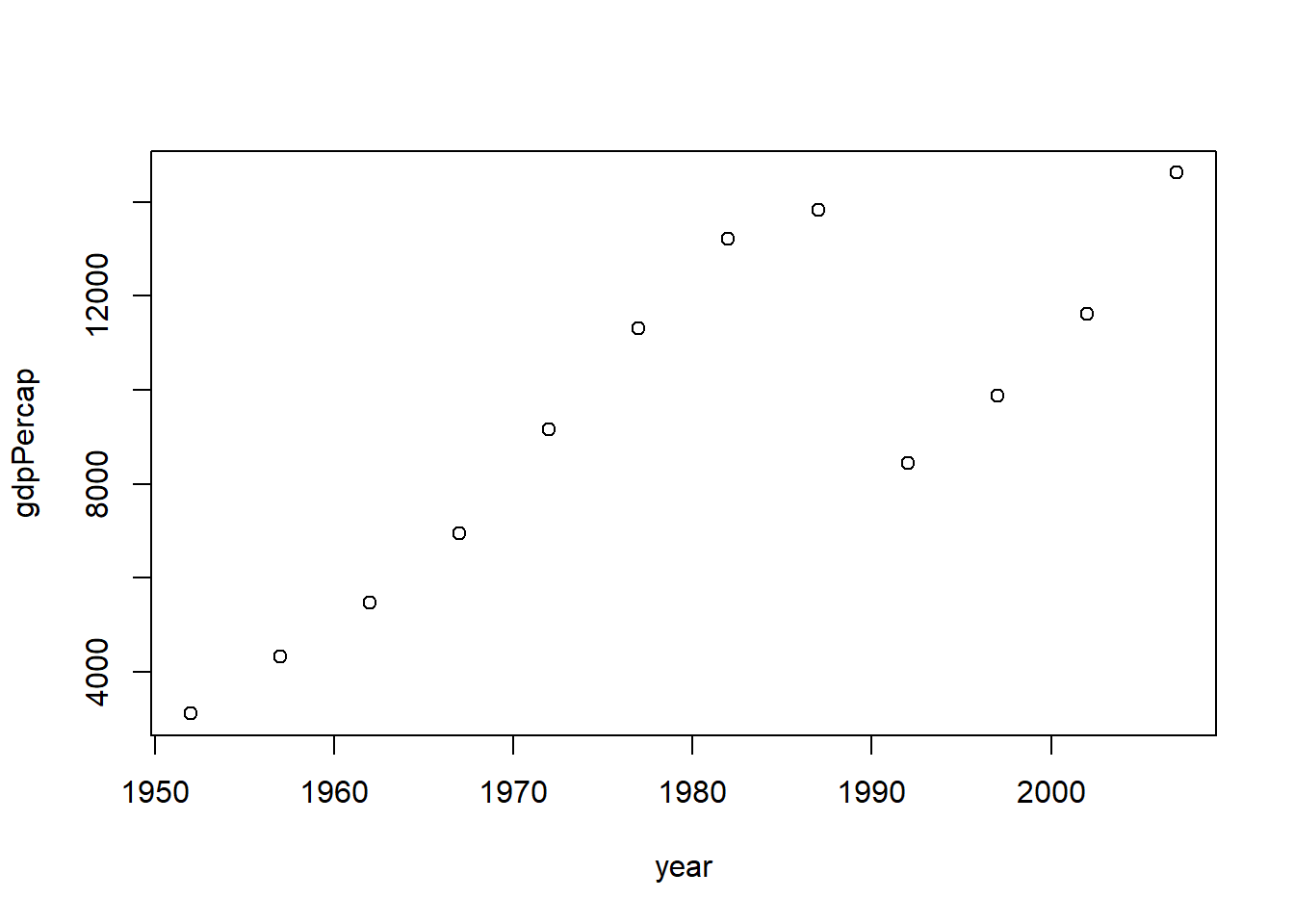
library (dplyr)%>% filter (country== "Croatia" ) %>% select (year, gdpPercap) %>% plot$ country == "Croatia" , ]
# A tibble: 12 × 6
   country continent  year lifeExp     pop gdpPercap
   <fct>   <fct>     <int>   <dbl>   <int>     <dbl>
 1 Croatia Europe     1952    61.2 3882229     3119.
 2 Croatia Europe     1957    64.8 3991242     4338.
 3 Croatia Europe     1962    67.1 4076557     5478.
 4 Croatia Europe     1967    68.5 4174366     6960.
 5 Croatia Europe     1972    69.6 4225310     9164.
 6 Croatia Europe     1977    70.6 4318673    11305.
 7 Croatia Europe     1982    70.5 4413368    13222.
 8 Croatia Europe     1987    71.5 4484310    13823.
 9 Croatia Europe     1992    72.5 4494013     8448.
10 Croatia Europe     1997    73.7 4444595     9876.
11 Croatia Europe     2002    74.9 4481020    11628.
12 Croatia Europe     2007    75.7 4493312    14619.
$ country == "Korea, Rep." , ]
# A tibble: 12 × 6
   country     continent  year lifeExp      pop gdpPercap
   <fct>       <fct>     <int>   <dbl>    <int>     <dbl>
 1 Korea, Rep. Asia       1952    47.5 20947571     1031.
 2 Korea, Rep. Asia       1957    52.7 22611552     1488.
 3 Korea, Rep. Asia       1962    55.3 26420307     1536.
 4 Korea, Rep. Asia       1967    57.7 30131000     2029.
 5 Korea, Rep. Asia       1972    62.6 33505000     3031.
 6 Korea, Rep. Asia       1977    64.8 36436000     4657.
 7 Korea, Rep. Asia       1982    67.1 39326000     5623.
 8 Korea, Rep. Asia       1987    69.8 41622000     8533.
 9 Korea, Rep. Asia       1992    72.2 43805450    12104.
10 Korea, Rep. Asia       1997    74.6 46173816    15994.
11 Korea, Rep. Asia       2002    77.0 47969150    19234.
12 Korea, Rep. Asia       2007    78.6 49044790    23348.
levels (gapminder$ country)
  [1] "Afghanistan"              "Albania"
  [3] "Algeria"                  "Angola"
  [5] "Argentina"                "Australia"
  [7] "Austria"                  "Bahrain"
  [9] "Bangladesh"               "Belgium"
 [11] "Benin"                    "Bolivia"
 [13] "Bosnia and Herzegovina"   "Botswana"
 [15] "Brazil"                   "Bulgaria"
 [17] "Burkina Faso"             "Burundi"
 [19] "Cambodia"                 "Cameroon"
 [21] "Canada"                   "Central African Republic"
 [23] "Chad"                     "Chile"
 [25] "China"                    "Colombia"
 [27] "Comoros"                  "Congo, Dem. Rep."
 [29] "Congo, Rep."              "Costa Rica"
 [31] "Cote d'Ivoire"            "Croatia"
 [33] "Cuba"                     "Czech Republic"
 [35] "Denmark"                  "Djibouti"
 [37] "Dominican Republic"       "Ecuador"
 [39] "Egypt"                    "El Salvador"
 [41] "Equatorial Guinea"        "Eritrea"
 [43] "Ethiopia"                 "Finland"
 [45] "France"                   "Gabon"
 [47] "Gambia"                   "Germany"
 [49] "Ghana"                    "Greece"
 [51] "Guatemala"                "Guinea"
 [53] "Guinea-Bissau"            "Haiti"
 [55] "Honduras"                 "Hong Kong, China"
 [57] "Hungary"                  "Iceland"
 [59] "India"                    "Indonesia"
 [61] "Iran"                     "Iraq"
 [63] "Ireland"                  "Israel"
 [65] "Italy"                    "Jamaica"
 [67] "Japan"                    "Jordan"
 [69] "Kenya"                    "Korea, Dem. Rep."
 [71] "Korea, Rep."              "Kuwait"
 [73] "Lebanon"                  "Lesotho"
 [75] "Liberia"                  "Libya"
 [77] "Madagascar"               "Malawi"
 [79] "Malaysia"                 "Mali"
 [81] "Mauritania"               "Mauritius"
 [83] "Mexico"                   "Mongolia"
 [85] "Montenegro"               "Morocco"
 [87] "Mozambique"               "Myanmar"
 [89] "Namibia"                  "Nepal"
 [91] "Netherlands"              "New Zealand"
 [93] "Nicaragua"                "Niger"
 [95] "Nigeria"                  "Norway"
 [97] "Oman"                     "Pakistan"
 [99] "Panama"                   "Paraguay"
[101] "Peru"                     "Philippines"
[103] "Poland"                   "Portugal"
[105] "Puerto Rico"              "Reunion"
[107] "Romania"                  "Rwanda"
[109] "Sao Tome and Principe"    "Saudi Arabia"
[111] "Senegal"                  "Serbia"
[113] "Sierra Leone"             "Singapore"
[115] "Slovak Republic"          "Slovenia"
[117] "Somalia"                  "South Africa"
[119] "Spain"                    "Sri Lanka"
[121] "Sudan"                    "Swaziland"
[123] "Sweden"                   "Switzerland"
[125] "Syria"                    "Taiwan"
[127] "Tanzania"                 "Thailand"
[129] "Togo"                     "Trinidad and Tobago"
[131] "Tunisia"                  "Turkey"
[133] "Uganda"                   "United Kingdom"
[135] "United States"            "Uruguay"
[137] "Venezuela"                "Vietnam"
[139] "West Bank and Gaza"       "Yemen, Rep."
[141] "Zambia"                   "Zimbabwe"
$ country == "Croatia" , "pop" ]
# A tibble: 12 × 1
       pop
     <int>
 1 3882229
 2 3991242
 3 4076557
 4 4174366
 5 4225310
 6 4318673
 7 4413368
 8 4484310
 9 4494013
10 4444595
11 4481020
12 4493312
$ country == "Croatia" , c ("lifeExp" ,"pop" )]
# A tibble: 12 × 2
   lifeExp     pop
     <dbl>   <int>
 1    61.2 3882229
 2    64.8 3991242
 3    67.1 4076557
 4    68.5 4174366
 5    69.6 4225310
 6    70.6 4318673
 7    70.5 4413368
 8    71.5 4484310
 9    72.5 4494013
10    73.7 4444595
11    74.9 4481020
12    75.7 4493312
$ country == "Croatia" & #Croatia extraction $ year > 1990 , #1990 after c ("lifeExp" ,"pop" )] # those variables
# A tibble: 4 × 2
  lifeExp     pop
    <dbl>   <int>
1    72.5 4494013
2    73.7 4444595
3    74.9 4481020
4    75.7 4493312
apply (gapminder[gapminder$ country == "Croatia" ,c ("lifeExp" ,"pop" )],2 , mean)
     lifeExp          pop
7.005592e+01 4.289916e+06
apply (gapminder[gapminder$ country == "Korea, Rep." ,c ("lifeExp" ,"pop" )],2 , mean)
     lifeExp          pop
      65.001 36499386.333
# 03 Data processing using the dplyr library # select (gapminder, country, year, lifeExp)
# A tibble: 1,704 × 3
   country      year lifeExp
   <fct>       <int>   <dbl>
 1 Afghanistan  1952    28.8
 2 Afghanistan  1957    30.3
 3 Afghanistan  1962    32.0
 4 Afghanistan  1967    34.0
 5 Afghanistan  1972    36.1
 6 Afghanistan  1977    38.4
 7 Afghanistan  1982    39.9
 8 Afghanistan  1987    40.8
 9 Afghanistan  1992    41.7
10 Afghanistan  1997    41.8
# ℹ 1,694 more rows
filter (gapminder, country == "Croatia" )
# A tibble: 12 × 6
   country continent  year lifeExp     pop gdpPercap
   <fct>   <fct>     <int>   <dbl>   <int>     <dbl>
 1 Croatia Europe     1952    61.2 3882229     3119.
 2 Croatia Europe     1957    64.8 3991242     4338.
 3 Croatia Europe     1962    67.1 4076557     5478.
 4 Croatia Europe     1967    68.5 4174366     6960.
 5 Croatia Europe     1972    69.6 4225310     9164.
 6 Croatia Europe     1977    70.6 4318673    11305.
 7 Croatia Europe     1982    70.5 4413368    13222.
 8 Croatia Europe     1987    71.5 4484310    13823.
 9 Croatia Europe     1992    72.5 4494013     8448.
10 Croatia Europe     1997    73.7 4444595     9876.
11 Croatia Europe     2002    74.9 4481020    11628.
12 Croatia Europe     2007    75.7 4493312    14619.
summarize (gapminder, pop_avg = mean (pop))
# A tibble: 1 × 1
    pop_avg
      <dbl>
1 29601212.
summarize (group_by (gapminder, continent), pop_avg = mean (pop))
# A tibble: 5 × 2
  continent   pop_avg
  <fct>         <dbl>
1 Africa     9916003.
2 Americas  24504795.
3 Asia      77038722.
4 Europe    17169765.
5 Oceania    8874672.
summarize (group_by (gapminder, continent, country), pop_avg = mean (pop))
`summarise()` has grouped output by 'continent'. You can override using the
`.groups` argument.
# A tibble: 142 × 3
# Groups:   continent [5]
   continent country                    pop_avg
   <fct>     <fct>                        <dbl>
 1 Africa    Algeria                  19875406.
 2 Africa    Angola                    7309390.
 3 Africa    Benin                     4017497.
 4 Africa    Botswana                   971186.
 5 Africa    Burkina Faso              7548677.
 6 Africa    Burundi                   4651608.
 7 Africa    Cameroon                  9816648.
 8 Africa    Central African Republic  2560963
 9 Africa    Chad                      5329256.
10 Africa    Comoros                    361684.
# ℹ 132 more rows
%>% group_by (continent, country) %>% summarize (pop_avg = mean (pop))
`summarise()` has grouped output by 'continent'. You can override using the
`.groups` argument.
# A tibble: 142 × 3
# Groups:   continent [5]
   continent country                    pop_avg
   <fct>     <fct>                        <dbl>
 1 Africa    Algeria                  19875406.
 2 Africa    Angola                    7309390.
 3 Africa    Benin                     4017497.
 4 Africa    Botswana                   971186.
 5 Africa    Burkina Faso              7548677.
 6 Africa    Burundi                   4651608.
 7 Africa    Cameroon                  9816648.
 8 Africa    Central African Republic  2560963
 9 Africa    Chad                      5329256.
10 Africa    Comoros                    361684.
# ℹ 132 more rows
= filter (gapminder, country == "Croatia" )= select (temp1, country, year, lifeExp)= apply (temp2[ , c ("lifeExp" )], 2 , mean)
%>% filter (country == "Croatia" ) %>% select (country, year, lifeExp) %>% summarize (lifeExp_avg = mean (lifeExp))
# A tibble: 1 × 1
  lifeExp_avg
        <dbl>
1        70.1
data in need: avocado.csv
# 04 The reality of data processing # library (ggplot2)<- read.csv ("data/avocado.csv" , header= TRUE , sep = "," )str (avocado)
'data.frame':   18249 obs. of  14 variables:
 $ X           : int  0 1 2 3 4 5 6 7 8 9 ...
 $ Date        : chr  "2015-12-27" "2015-12-20" "2015-12-13" "2015-12-06" ...
 $ AveragePrice: num  1.33 1.35 0.93 1.08 1.28 1.26 0.99 0.98 1.02 1.07 ...
 $ Total.Volume: num  64237 54877 118220 78992 51040 ...
 $ X4046       : num  1037 674 795 1132 941 ...
 $ X4225       : num  54455 44639 109150 71976 43838 ...
 $ X4770       : num  48.2 58.3 130.5 72.6 75.8 ...
 $ Total.Bags  : num  8697 9506 8145 5811 6184 ...
 $ Small.Bags  : num  8604 9408 8042 5677 5986 ...
 $ Large.Bags  : num  93.2 97.5 103.1 133.8 197.7 ...
 $ XLarge.Bags : num  0 0 0 0 0 0 0 0 0 0 ...
 $ type        : chr  "conventional" "conventional" "conventional" "conventional" ...
 $ year        : int  2015 2015 2015 2015 2015 2015 2015 2015 2015 2015 ...
 $ region      : chr  "Albany" "Albany" "Albany" "Albany" ...
x_avg = avocado %>% group_by (region) %>% summarize (V_avg = mean (Total.Volume), P_avg = mean (AveragePrice)))
# A tibble: 54 × 3
   region                 V_avg P_avg
   <chr>                  <dbl> <dbl>
 1 Albany                47538.  1.56
 2 Atlanta              262145.  1.34
 3 BaltimoreWashington  398562.  1.53
 4 Boise                 42643.  1.35
 5 Boston               287793.  1.53
 6 BuffaloRochester      67936.  1.52
 7 California          3044324.  1.40
 8 Charlotte            105194.  1.61
 9 Chicago              395569.  1.56
10 CincinnatiDayton     131722.  1.21
# ℹ 44 more rows
x_avg = avocado %>% group_by (region, year) %>% summarize (V_avg = mean (Total.Volume), P_avg = mean (AveragePrice)))
`summarise()` has grouped output by 'region'. You can override using the
`.groups` argument.
# A tibble: 216 × 4
# Groups:   region [54]
   region               year   V_avg P_avg
   <chr>               <int>   <dbl> <dbl>
 1 Albany               2015  38749.  1.54
 2 Albany               2016  50619.  1.53
 3 Albany               2017  49355.  1.64
 4 Albany               2018  64249.  1.44
 5 Atlanta              2015 223382.  1.38
 6 Atlanta              2016 272374.  1.21
 7 Atlanta              2017 271841.  1.43
 8 Atlanta              2018 342976.  1.29
 9 BaltimoreWashington  2015 390823.  1.37
10 BaltimoreWashington  2016 393210.  1.59
# ℹ 206 more rows
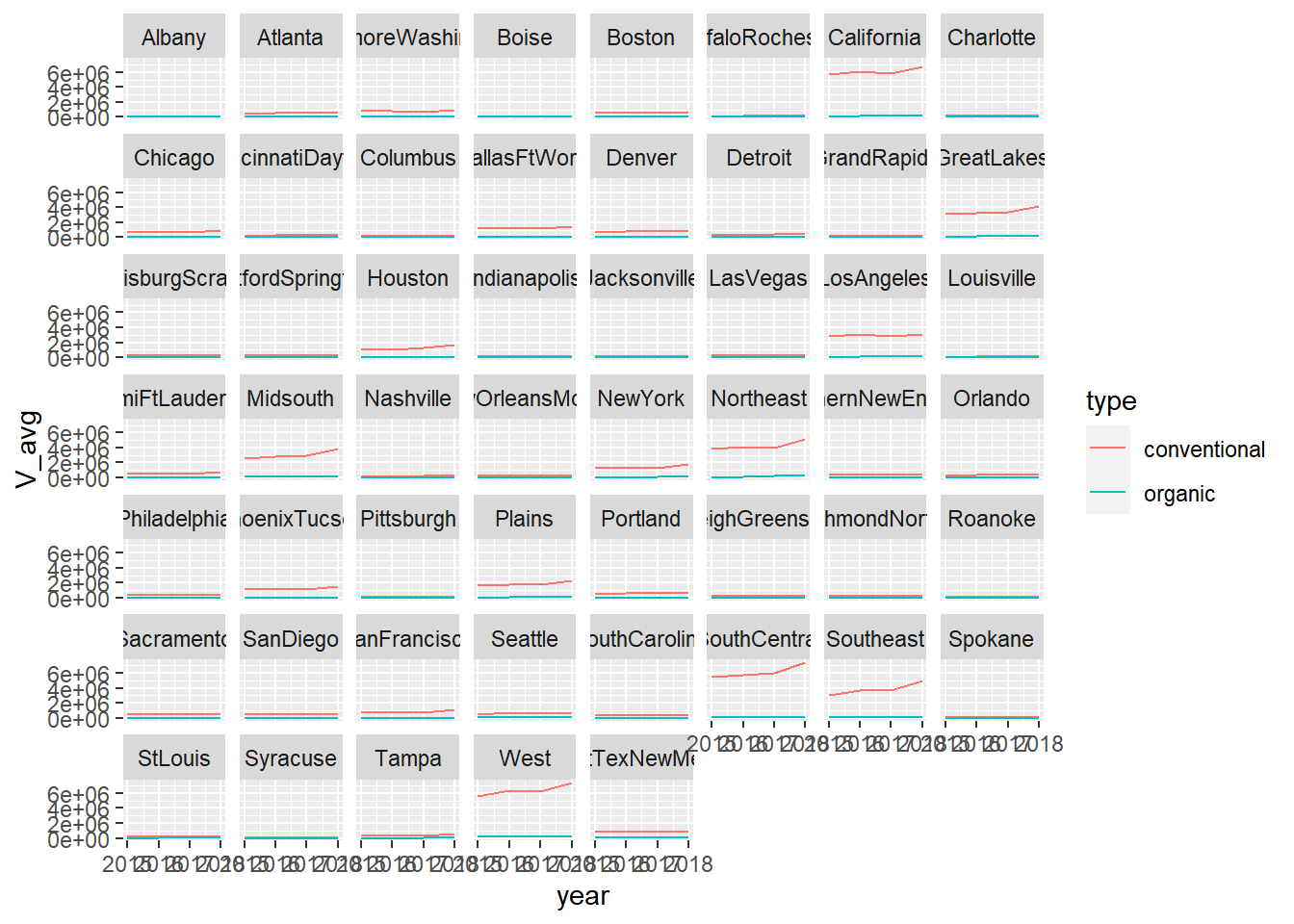
= avocado %>% group_by (region, year, type) %>% summarize (V_avg = mean (Total.Volume), P_avg = mean (AveragePrice))
`summarise()` has grouped output by 'region', 'year'. You can override using
the `.groups` argument.
%>% group_by (region, year, type) %>% summarize (V_avg = mean (Total.Volume),P_avg = mean (AveragePrice)) -> x_avg
`summarise()` has grouped output by 'region', 'year'. You can override using
the `.groups` argument.
%>% filter (region != "TotalUS" ) %>% ggplot (aes (year, V_avg, col = type)) + geom_line () + facet_wrap (~ region)
# install.packages("ggplot2") library (ggplot2)arrange (x_avg, desc (V_avg))
# A tibble: 432 × 5
# Groups:   region, year [216]
   region        year type             V_avg P_avg
   <chr>        <int> <chr>            <dbl> <dbl>
 1 TotalUS       2018 conventional 42125533. 1.06
 2 TotalUS       2016 conventional 34043450. 1.05
 3 TotalUS       2017 conventional 33995658. 1.22
 4 TotalUS       2015 conventional 31224729. 1.01
 5 SouthCentral  2018 conventional  7465557. 0.806
 6 West          2018 conventional  7451445. 0.981
 7 California    2018 conventional  6786962. 1.08
 8 West          2016 conventional  6404892. 0.916
 9 West          2017 conventional  6279482. 1.10
10 California    2016 conventional  6105539. 1.05
# ℹ 422 more rows
= x_avg %>% filter (region != "TotalUS" )
# After excluding TotalUS, you can process it using statistical functions directly. $ V_avg == max (x_avg1$ V_avg),]
# A tibble: 1 × 5
# Groups:   region, year [1]
  region        year type            V_avg P_avg
  <chr>        <int> <chr>           <dbl> <dbl>
1 SouthCentral  2018 conventional 7465557. 0.806
# install.packages("lubridate") library (lubridate)
Attaching package: 'lubridate'
The following objects are masked from 'package:base':

    date, intersect, setdiff, union
x_avg = avocado %>% group_by (region, year, month (Date), type) %>% summarize (V_avg = mean (Total.Volume), P_avg = mean (AveragePrice)))
`summarise()` has grouped output by 'region', 'year', 'month(Date)'. You can
override using the `.groups` argument.
# A tibble: 4,212 × 6
# Groups:   region, year, month(Date) [2,106]
   region  year `month(Date)` type          V_avg P_avg
   <chr>  <int>         <dbl> <chr>         <dbl> <dbl>
 1 Albany  2015             1 conventional 42932.  1.17
 2 Albany  2015             1 organic       1198.  1.84
 3 Albany  2015             2 conventional 52343.  1.03
 4 Albany  2015             2 organic       1334.  1.76
 5 Albany  2015             3 conventional 50659.  1.06
 6 Albany  2015             3 organic       1444.  1.83
 7 Albany  2015             4 conventional 48594.  1.17
 8 Albany  2015             4 organic       1402.  1.89
 9 Albany  2015             5 conventional 97216.  1.26
10 Albany  2015             5 organic       1836.  1.94
# ℹ 4,202 more rows
Class
Introduction to Tidyverse
The tidyverse is a powerful collection of R packages that are actually data tools for transforming and visualizing data. All packages of the tidyverse share an underlying philosophy and common APls.
The core packages are:
ggplot2, which implements the grammar of graphics. You can use it to visualize your data.
dplyr is a grammar of data You can use it to solve the most common data manipulation challenges.
tidyr helps you to create tidy data or data where each variable is in a column, each observation is a row end each value is a column, each observation is a row end each value is a cell.
readr is a fast and friendly way to read rectangular
purrr enhances R’s functional programming (FP)toolkit by providing a complete and consistent set of tools for working with functions and vectors.
tibble is a modern re-imaginging of the data
stringr provides a cohesive set of functions designed to make working with strings as easy as possible
forcats provide a suite of useful tools that solve common problems with factors.
tidyverse
Before Tidyverse Before the tidyverse, R programming was largely centered around base R functions and packages. This included using base R functions for data manipulation (like subsetmergeapplyplothist
After Tidyverse The tidyverse, developed by Hadley Wickham and others, brought a suite of packages designed to work harmoniously together using a consistent syntax and underlying philosophy. Key features and impacts include:
Consistent Syntax : The tidyverse introduced a consistent and readable syntax that leverages chaining operations using the %>%magrittr
Data Manipulation : With dplyrfilter()arrange()select()mutate()summarise()
Data Importing and Tidying : readrtidyr
Visualization : ggplot2
Community and Accessibility : The tidyverse has fostered a strong community and has contributed significantly to teaching materials that are user-friendly and accessible to beginners. This has democratized data analysis in R, making it more accessible to non-programmers.
Impact on Package Development : The tidyverse’s philosophy and popularity have influenced the development of other packages, even those not part of the tidyverse, to adopt tidy principles and interoperate smoothly with tidyverse packages.
The tidyverse has not only changed the syntax and functionality of R coding but also its philosophy towards data analysis. It promotes a workflow that is coherent, transparent, and efficient, which has been widely adopted in academia, industry, and teaching. While some veteran R users prefer the flexibility and control of base R, the tidyverse’s approachable syntax and powerful capabilities have made it a pivotal tool in modern R programming, particularly for data science.
Please check out the homepage of tidyverse: https://www.tidyverse.org/
You can install the complete tidyverse with:
> install.packages(“tidyverse”)
Then, load the core tidyverse and make it available in your current R session by running:
> library(tidyverse)
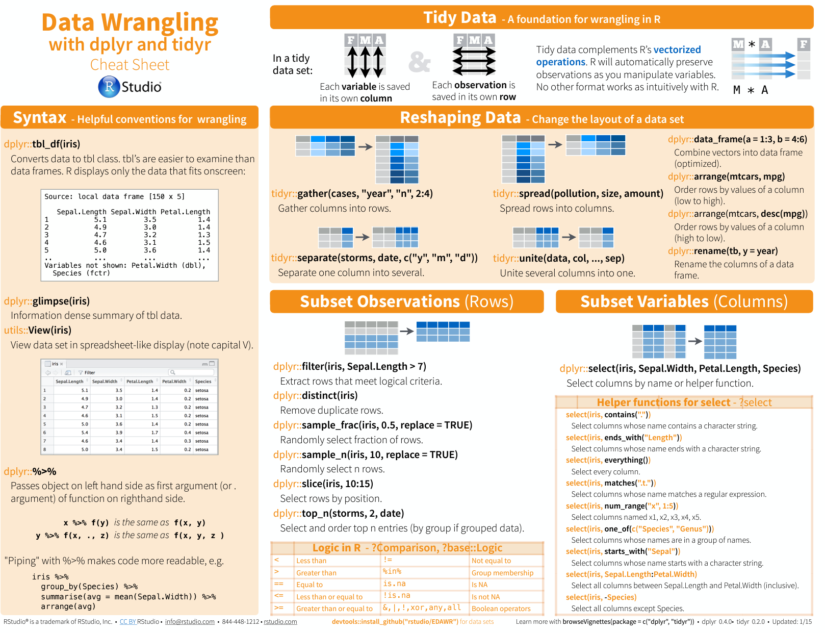
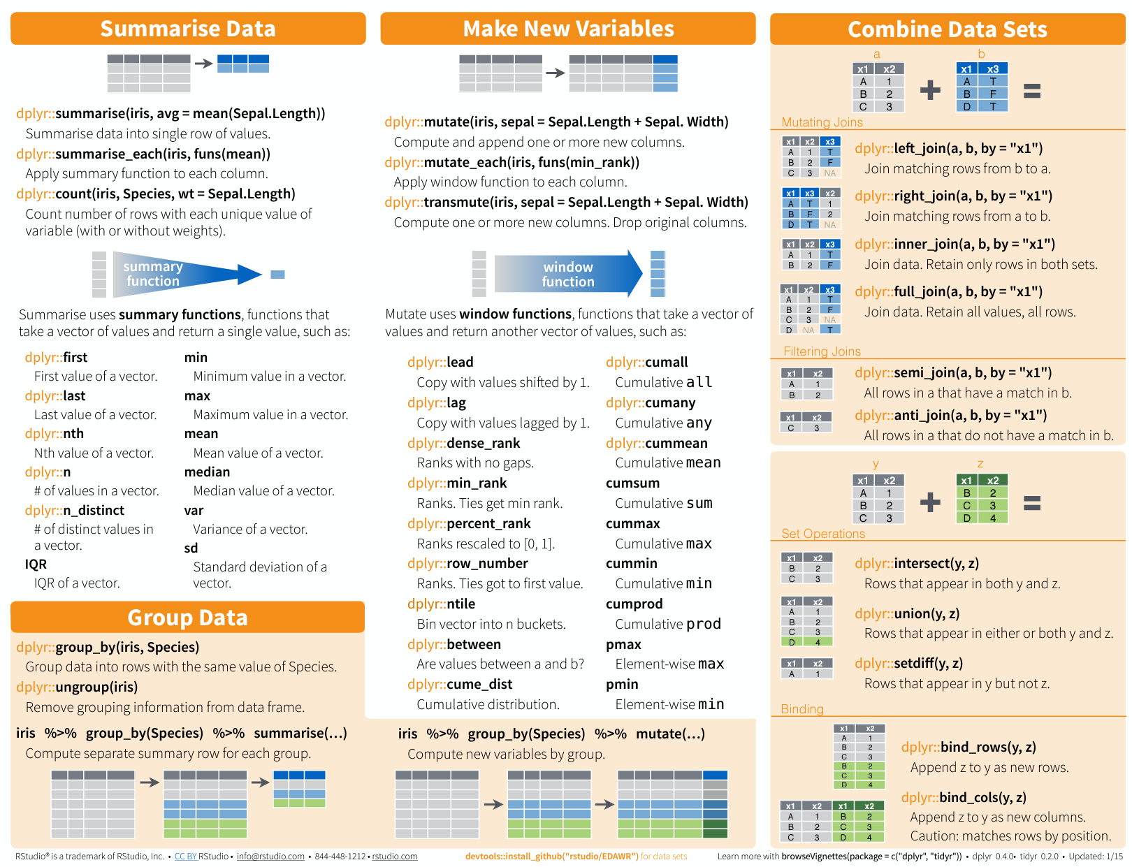
Please see this cheat sheet:
https://www.rstudio.com/wp-content/uploads/2015/02/data-wrangling-cheatsheet.pdf
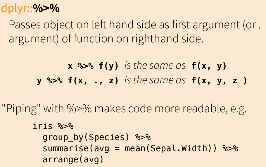
Pipe
Subset Observations
# filter %>% filter (Sepal.Length > 7 )
   Sepal.Length Sepal.Width Petal.Length Petal.Width   Species
1           7.1         3.0          5.9         2.1 virginica
2           7.6         3.0          6.6         2.1 virginica
3           7.3         2.9          6.3         1.8 virginica
4           7.2         3.6          6.1         2.5 virginica
5           7.7         3.8          6.7         2.2 virginica
6           7.7         2.6          6.9         2.3 virginica
7           7.7         2.8          6.7         2.0 virginica
8           7.2         3.2          6.0         1.8 virginica
9           7.2         3.0          5.8         1.6 virginica
10          7.4         2.8          6.1         1.9 virginica
11          7.9         3.8          6.4         2.0 virginica
12          7.7         3.0          6.1         2.3 virginica
[1] "setosa" "versicolor" "virginica"
%>% filter (Species == "setosa" )
   Sepal.Length Sepal.Width Petal.Length Petal.Width Species
1           5.1         3.5          1.4         0.2  setosa
2           4.9         3.0          1.4         0.2  setosa
3           4.7         3.2          1.3         0.2  setosa
4           4.6         3.1          1.5         0.2  setosa
5           5.0         3.6          1.4         0.2  setosa
6           5.4         3.9          1.7         0.4  setosa
7           4.6         3.4          1.4         0.3  setosa
8           5.0         3.4          1.5         0.2  setosa
9           4.4         2.9          1.4         0.2  setosa
10          4.9         3.1          1.5         0.1  setosa
11          5.4         3.7          1.5         0.2  setosa
12          4.8         3.4          1.6         0.2  setosa
13          4.8         3.0          1.4         0.1  setosa
14          4.3         3.0          1.1         0.1  setosa
15          5.8         4.0          1.2         0.2  setosa
16          5.7         4.4          1.5         0.4  setosa
17          5.4         3.9          1.3         0.4  setosa
18          5.1         3.5          1.4         0.3  setosa
19          5.7         3.8          1.7         0.3  setosa
20          5.1         3.8          1.5         0.3  setosa
21          5.4         3.4          1.7         0.2  setosa
22          5.1         3.7          1.5         0.4  setosa
23          4.6         3.6          1.0         0.2  setosa
24          5.1         3.3          1.7         0.5  setosa
25          4.8         3.4          1.9         0.2  setosa
26          5.0         3.0          1.6         0.2  setosa
27          5.0         3.4          1.6         0.4  setosa
28          5.2         3.5          1.5         0.2  setosa
29          5.2         3.4          1.4         0.2  setosa
30          4.7         3.2          1.6         0.2  setosa
31          4.8         3.1          1.6         0.2  setosa
32          5.4         3.4          1.5         0.4  setosa
33          5.2         4.1          1.5         0.1  setosa
34          5.5         4.2          1.4         0.2  setosa
35          4.9         3.1          1.5         0.2  setosa
36          5.0         3.2          1.2         0.2  setosa
37          5.5         3.5          1.3         0.2  setosa
38          4.9         3.6          1.4         0.1  setosa
39          4.4         3.0          1.3         0.2  setosa
40          5.1         3.4          1.5         0.2  setosa
41          5.0         3.5          1.3         0.3  setosa
42          4.5         2.3          1.3         0.3  setosa
43          4.4         3.2          1.3         0.2  setosa
44          5.0         3.5          1.6         0.6  setosa
45          5.1         3.8          1.9         0.4  setosa
46          4.8         3.0          1.4         0.3  setosa
47          5.1         3.8          1.6         0.2  setosa
48          4.6         3.2          1.4         0.2  setosa
49          5.3         3.7          1.5         0.2  setosa
50          5.0         3.3          1.4         0.2  setosa
%>% filter (Species == "setosa" ) %>% plot%>% filter (Species == "setosa" ) %>% summary
  Sepal.Length    Sepal.Width     Petal.Length    Petal.Width
 Min.   :4.300   Min.   :2.300   Min.   :1.000   Min.   :0.100
 1st Qu.:4.800   1st Qu.:3.200   1st Qu.:1.400   1st Qu.:0.200
 Median :5.000   Median :3.400   Median :1.500   Median :0.200
 Mean   :5.006   Mean   :3.428   Mean   :1.462   Mean   :0.246
 3rd Qu.:5.200   3rd Qu.:3.675   3rd Qu.:1.575   3rd Qu.:0.300
 Max.   :5.800   Max.   :4.400   Max.   :1.900   Max.   :0.600
       Species
 setosa    :50
 versicolor: 0
 virginica : 0
# distinct: remove duplication (take only unique values) %>% distinct (Species)
     Species
1     setosa
2 versicolor
3  virginica
# random sampling %>% nrow%>% sample_frac (0.5 , replace= T)
   Sepal.Length Sepal.Width Petal.Length Petal.Width    Species
1           5.2         4.1          1.5         0.1     setosa
2           6.5         3.2          5.1         2.0  virginica
3           6.5         2.8          4.6         1.5 versicolor
4           6.1         3.0          4.6         1.4 versicolor
5           5.7         2.6          3.5         1.0 versicolor
6           6.5         3.0          5.5         1.8  virginica
7           7.2         3.6          6.1         2.5  virginica
8           6.3         2.5          5.0         1.9  virginica
9           4.3         3.0          1.1         0.1     setosa
10          4.6         3.6          1.0         0.2     setosa
11          5.6         2.9          3.6         1.3 versicolor
12          7.6         3.0          6.6         2.1  virginica
13          6.3         2.5          4.9         1.5 versicolor
14          4.6         3.6          1.0         0.2     setosa
15          7.4         2.8          6.1         1.9  virginica
16          6.4         2.8          5.6         2.1  virginica
17          5.5         2.6          4.4         1.2 versicolor
18          7.7         3.0          6.1         2.3  virginica
19          6.4         3.1          5.5         1.8  virginica
20          6.3         2.5          4.9         1.5 versicolor
21          6.2         2.2          4.5         1.5 versicolor
22          5.8         2.7          4.1         1.0 versicolor
23          6.9         3.2          5.7         2.3  virginica
24          6.7         2.5          5.8         1.8  virginica
25          4.8         3.4          1.6         0.2     setosa
26          5.7         4.4          1.5         0.4     setosa
27          5.8         4.0          1.2         0.2     setosa
28          7.7         2.6          6.9         2.3  virginica
29          6.9         3.1          5.1         2.3  virginica
30          7.7         3.0          6.1         2.3  virginica
31          4.8         3.4          1.9         0.2     setosa
32          6.8         3.2          5.9         2.3  virginica
33          5.1         2.5          3.0         1.1 versicolor
34          7.9         3.8          6.4         2.0  virginica
35          6.3         3.4          5.6         2.4  virginica
36          4.9         3.1          1.5         0.2     setosa
37          5.9         3.0          4.2         1.5 versicolor
38          6.1         2.8          4.7         1.2 versicolor
39          5.1         3.8          1.9         0.4     setosa
40          6.9         3.1          4.9         1.5 versicolor
41          5.4         3.4          1.5         0.4     setosa
42          6.3         2.7          4.9         1.8  virginica
43          5.2         2.7          3.9         1.4 versicolor
44          5.7         3.0          4.2         1.2 versicolor
45          5.5         2.5          4.0         1.3 versicolor
46          6.7         3.3          5.7         2.1  virginica
47          5.6         2.5          3.9         1.1 versicolor
48          4.9         3.1          1.5         0.2     setosa
49          6.1         2.9          4.7         1.4 versicolor
50          6.5         2.8          4.6         1.5 versicolor
51          5.4         3.0          4.5         1.5 versicolor
52          5.0         3.3          1.4         0.2     setosa
53          4.4         3.2          1.3         0.2     setosa
54          6.4         2.8          5.6         2.1  virginica
55          5.0         2.0          3.5         1.0 versicolor
56          5.5         2.4          3.8         1.1 versicolor
57          6.3         3.3          4.7         1.6 versicolor
58          4.9         3.0          1.4         0.2     setosa
59          5.0         3.5          1.3         0.3     setosa
60          6.2         2.8          4.8         1.8  virginica
61          6.8         3.2          5.9         2.3  virginica
62          5.1         3.8          1.6         0.2     setosa
63          4.8         3.0          1.4         0.1     setosa
64          6.3         2.8          5.1         1.5  virginica
65          5.7         2.8          4.1         1.3 versicolor
66          6.6         3.0          4.4         1.4 versicolor
67          6.7         3.1          4.7         1.5 versicolor
68          7.2         3.2          6.0         1.8  virginica
69          6.6         3.0          4.4         1.4 versicolor
70          7.7         2.6          6.9         2.3  virginica
71          6.7         3.1          4.7         1.5 versicolor
72          7.2         3.0          5.8         1.6  virginica
73          6.9         3.1          5.1         2.3  virginica
74          6.7         3.1          5.6         2.4  virginica
75          7.6         3.0          6.6         2.1  virginica
%>% sample_frac (0.5 , replace= T) %>% nrow%>% sample_n (10 , replace= T)
   Sepal.Length Sepal.Width Petal.Length Petal.Width    Species
1           5.6         3.0          4.5         1.5 versicolor
2           6.8         3.2          5.9         2.3  virginica
3           5.6         2.5          3.9         1.1 versicolor
4           6.3         2.9          5.6         1.8  virginica
5           6.3         2.3          4.4         1.3 versicolor
6           6.0         3.0          4.8         1.8  virginica
7           5.1         3.8          1.6         0.2     setosa
8           5.2         3.5          1.5         0.2     setosa
9           7.6         3.0          6.6         2.1  virginica
10          5.1         3.5          1.4         0.2     setosa
%>% sample_n (10 , replace= T) %>% nrow # slice %>% slice (10 : 15 )
  Sepal.Length Sepal.Width Petal.Length Petal.Width Species
1          4.9         3.1          1.5         0.1  setosa
2          5.4         3.7          1.5         0.2  setosa
3          4.8         3.4          1.6         0.2  setosa
4          4.8         3.0          1.4         0.1  setosa
5          4.3         3.0          1.1         0.1  setosa
6          5.8         4.0          1.2         0.2  setosa
# Top n in X %>% top_n (5 , Sepal.Length)
  Sepal.Length Sepal.Width Petal.Length Petal.Width   Species
1          7.7         3.8          6.7         2.2 virginica
2          7.7         2.6          6.9         2.3 virginica
3          7.7         2.8          6.7         2.0 virginica
4          7.9         3.8          6.4         2.0 virginica
5          7.7         3.0          6.1         2.3 virginica
%>% top_n (5 , Sepal.Width)
  Sepal.Length Sepal.Width Petal.Length Petal.Width Species
1          5.4         3.9          1.7         0.4  setosa
2          5.8         4.0          1.2         0.2  setosa
3          5.7         4.4          1.5         0.4  setosa
4          5.4         3.9          1.3         0.4  setosa
5          5.2         4.1          1.5         0.1  setosa
6          5.5         4.2          1.4         0.2  setosa
Subset Variables
# pull & select %>% pull (Petal.Width)
  [1] 0.2 0.2 0.2 0.2 0.2 0.4 0.3 0.2 0.2 0.1 0.2 0.2 0.1 0.1 0.2 0.4 0.4 0.3
 [19] 0.3 0.3 0.2 0.4 0.2 0.5 0.2 0.2 0.4 0.2 0.2 0.2 0.2 0.4 0.1 0.2 0.2 0.2
 [37] 0.2 0.1 0.2 0.2 0.3 0.3 0.2 0.6 0.4 0.3 0.2 0.2 0.2 0.2 1.4 1.5 1.5 1.3
 [55] 1.5 1.3 1.6 1.0 1.3 1.4 1.0 1.5 1.0 1.4 1.3 1.4 1.5 1.0 1.5 1.1 1.8 1.3
 [73] 1.5 1.2 1.3 1.4 1.4 1.7 1.5 1.0 1.1 1.0 1.2 1.6 1.5 1.6 1.5 1.3 1.3 1.3
 [91] 1.2 1.4 1.2 1.0 1.3 1.2 1.3 1.3 1.1 1.3 2.5 1.9 2.1 1.8 2.2 2.1 1.7 1.8
[109] 1.8 2.5 2.0 1.9 2.1 2.0 2.4 2.3 1.8 2.2 2.3 1.5 2.3 2.0 2.0 1.8 2.1 1.8
[127] 1.8 1.8 2.1 1.6 1.9 2.0 2.2 1.5 1.4 2.3 2.4 1.8 1.8 2.1 2.4 2.3 1.9 2.3
[145] 2.5 2.3 1.9 2.0 2.3 1.8
%>% select (Petal.Width)
    Petal.Width
1           0.2
2           0.2
3           0.2
4           0.2
5           0.2
6           0.4
7           0.3
8           0.2
9           0.2
10          0.1
11          0.2
12          0.2
13          0.1
14          0.1
15          0.2
16          0.4
17          0.4
18          0.3
19          0.3
20          0.3
21          0.2
22          0.4
23          0.2
24          0.5
25          0.2
26          0.2
27          0.4
28          0.2
29          0.2
30          0.2
31          0.2
32          0.4
33          0.1
34          0.2
35          0.2
36          0.2
37          0.2
38          0.1
39          0.2
40          0.2
41          0.3
42          0.3
43          0.2
44          0.6
45          0.4
46          0.3
47          0.2
48          0.2
49          0.2
50          0.2
51          1.4
52          1.5
53          1.5
54          1.3
55          1.5
56          1.3
57          1.6
58          1.0
59          1.3
60          1.4
61          1.0
62          1.5
63          1.0
64          1.4
65          1.3
66          1.4
67          1.5
68          1.0
69          1.5
70          1.1
71          1.8
72          1.3
73          1.5
74          1.2
75          1.3
76          1.4
77          1.4
78          1.7
79          1.5
80          1.0
81          1.1
82          1.0
83          1.2
84          1.6
85          1.5
86          1.6
87          1.5
88          1.3
89          1.3
90          1.3
91          1.2
92          1.4
93          1.2
94          1.0
95          1.3
96          1.2
97          1.3
98          1.3
99          1.1
100         1.3
101         2.5
102         1.9
103         2.1
104         1.8
105         2.2
106         2.1
107         1.7
108         1.8
109         1.8
110         2.5
111         2.0
112         1.9
113         2.1
114         2.0
115         2.4
116         2.3
117         1.8
118         2.2
119         2.3
120         1.5
121         2.3
122         2.0
123         2.0
124         1.8
125         2.1
126         1.8
127         1.8
128         1.8
129         2.1
130         1.6
131         1.9
132         2.0
133         2.2
134         1.5
135         1.4
136         2.3
137         2.4
138         1.8
139         1.8
140         2.1
141         2.4
142         2.3
143         1.9
144         2.3
145         2.5
146         2.3
147         1.9
148         2.0
149         2.3
150         1.8
%>% pull (Petal.Width) %>% str
num [1:150] 0.2 0.2 0.2 0.2 0.2 0.4 0.3 0.2 0.2 0.1 ...
%>% select (Petal.Width) %>% str
'data.frame':   150 obs. of  1 variable:
 $ Petal.Width: num  0.2 0.2 0.2 0.2 0.2 0.4 0.3 0.2 0.2 0.1 ...
%>% select (Petal.Length, Petal.Width) %>% head
  Petal.Length Petal.Width
1          1.4         0.2
2          1.4         0.2
3          1.3         0.2
4          1.5         0.2
5          1.4         0.2
6          1.7         0.4
# useful helpers: starts_with(), contains() %>% select (starts_with ("Peta" )) %>% head
  Petal.Length Petal.Width
1          1.4         0.2
2          1.4         0.2
3          1.3         0.2
4          1.5         0.2
5          1.4         0.2
6          1.7         0.4
%>% select (contains ("tal" )) %>% head
  Petal.Length Petal.Width
1          1.4         0.2
2          1.4         0.2
3          1.3         0.2
4          1.5         0.2
5          1.4         0.2
6          1.7         0.4
Reshaping & Arrange data
# let's use mtcars dataset
                     mpg cyl  disp  hp drat    wt  qsec vs am gear carb
Mazda RX4           21.0   6 160.0 110 3.90 2.620 16.46  0  1    4    4
Mazda RX4 Wag       21.0   6 160.0 110 3.90 2.875 17.02  0  1    4    4
Datsun 710          22.8   4 108.0  93 3.85 2.320 18.61  1  1    4    1
Hornet 4 Drive      21.4   6 258.0 110 3.08 3.215 19.44  1  0    3    1
Hornet Sportabout   18.7   8 360.0 175 3.15 3.440 17.02  0  0    3    2
Valiant             18.1   6 225.0 105 2.76 3.460 20.22  1  0    3    1
Duster 360          14.3   8 360.0 245 3.21 3.570 15.84  0  0    3    4
Merc 240D           24.4   4 146.7  62 3.69 3.190 20.00  1  0    4    2
Merc 230            22.8   4 140.8  95 3.92 3.150 22.90  1  0    4    2
Merc 280            19.2   6 167.6 123 3.92 3.440 18.30  1  0    4    4
Merc 280C           17.8   6 167.6 123 3.92 3.440 18.90  1  0    4    4
Merc 450SE          16.4   8 275.8 180 3.07 4.070 17.40  0  0    3    3
Merc 450SL          17.3   8 275.8 180 3.07 3.730 17.60  0  0    3    3
Merc 450SLC         15.2   8 275.8 180 3.07 3.780 18.00  0  0    3    3
Cadillac Fleetwood  10.4   8 472.0 205 2.93 5.250 17.98  0  0    3    4
Lincoln Continental 10.4   8 460.0 215 3.00 5.424 17.82  0  0    3    4
Chrysler Imperial   14.7   8 440.0 230 3.23 5.345 17.42  0  0    3    4
Fiat 128            32.4   4  78.7  66 4.08 2.200 19.47  1  1    4    1
Honda Civic         30.4   4  75.7  52 4.93 1.615 18.52  1  1    4    2
Toyota Corolla      33.9   4  71.1  65 4.22 1.835 19.90  1  1    4    1
Toyota Corona       21.5   4 120.1  97 3.70 2.465 20.01  1  0    3    1
Dodge Challenger    15.5   8 318.0 150 2.76 3.520 16.87  0  0    3    2
AMC Javelin         15.2   8 304.0 150 3.15 3.435 17.30  0  0    3    2
Camaro Z28          13.3   8 350.0 245 3.73 3.840 15.41  0  0    3    4
Pontiac Firebird    19.2   8 400.0 175 3.08 3.845 17.05  0  0    3    2
Fiat X1-9           27.3   4  79.0  66 4.08 1.935 18.90  1  1    4    1
Porsche 914-2       26.0   4 120.3  91 4.43 2.140 16.70  0  1    5    2
Lotus Europa        30.4   4  95.1 113 3.77 1.513 16.90  1  1    5    2
Ford Pantera L      15.8   8 351.0 264 4.22 3.170 14.50  0  1    5    4
Ferrari Dino        19.7   6 145.0 175 3.62 2.770 15.50  0  1    5    6
Maserati Bora       15.0   8 301.0 335 3.54 3.570 14.60  0  1    5    8
Volvo 142E          21.4   4 121.0 109 4.11 2.780 18.60  1  1    4    2
# About mtcars dataset # help(mtcars) # arrange %>% arrange (mpg) %>% head
                     mpg cyl disp  hp drat    wt  qsec vs am gear carb
Cadillac Fleetwood  10.4   8  472 205 2.93 5.250 17.98  0  0    3    4
Lincoln Continental 10.4   8  460 215 3.00 5.424 17.82  0  0    3    4
Camaro Z28          13.3   8  350 245 3.73 3.840 15.41  0  0    3    4
Duster 360          14.3   8  360 245 3.21 3.570 15.84  0  0    3    4
Chrysler Imperial   14.7   8  440 230 3.23 5.345 17.42  0  0    3    4
Maserati Bora       15.0   8  301 335 3.54 3.570 14.60  0  1    5    8
%>% add_rownames %>% head
Warning: `add_rownames()` was deprecated in dplyr 1.0.0.
ℹ Please use `tibble::rownames_to_column()` instead.
# A tibble: 6 × 12
  rowname        mpg   cyl  disp    hp  drat    wt  qsec    vs    am  gear  carb
  <chr>        <dbl> <dbl> <dbl> <dbl> <dbl> <dbl> <dbl> <dbl> <dbl> <dbl> <dbl>
1 Mazda RX4     21       6   160   110  3.9   2.62  16.5     0     1     4     4
2 Mazda RX4 W…  21       6   160   110  3.9   2.88  17.0     0     1     4     4
3 Datsun 710    22.8     4   108    93  3.85  2.32  18.6     1     1     4     1
4 Hornet 4 Dr…  21.4     6   258   110  3.08  3.22  19.4     1     0     3     1
5 Hornet Spor…  18.7     8   360   175  3.15  3.44  17.0     0     0     3     2
6 Valiant       18.1     6   225   105  2.76  3.46  20.2     1     0     3     1
%>% add_rownames %>% arrange (mpg) %>%
Warning: `add_rownames()` was deprecated in dplyr 1.0.0.
ℹ Please use `tibble::rownames_to_column()` instead.
# A tibble: 6 × 12
  rowname        mpg   cyl  disp    hp  drat    wt  qsec    vs    am  gear  carb
  <chr>        <dbl> <dbl> <dbl> <dbl> <dbl> <dbl> <dbl> <dbl> <dbl> <dbl> <dbl>
1 Cadillac Fl…  10.4     8   472   205  2.93  5.25  18.0     0     0     3     4
2 Lincoln Con…  10.4     8   460   215  3     5.42  17.8     0     0     3     4
3 Camaro Z28    13.3     8   350   245  3.73  3.84  15.4     0     0     3     4
4 Duster 360    14.3     8   360   245  3.21  3.57  15.8     0     0     3     4
5 Chrysler Im…  14.7     8   440   230  3.23  5.34  17.4     0     0     3     4
6 Maserati Bo…  15       8   301   335  3.54  3.57  14.6     0     1     5     8
%>% add_rownames %>% arrange (desc (mpg)) %>% select (rowname)
Warning: `add_rownames()` was deprecated in dplyr 1.0.0.
ℹ Please use `tibble::rownames_to_column()` instead.
# A tibble: 32 × 1
   rowname
   <chr>
 1 Toyota Corolla
 2 Fiat 128
 3 Honda Civic
 4 Lotus Europa
 5 Fiat X1-9
 6 Porsche 914-2
 7 Merc 240D
 8 Datsun 710
 9 Merc 230
10 Toyota Corona
# ℹ 22 more rows
Summarise data
# Summarise %>% summarise (avg.PL= mean (Petal.Length))%>% summarise (sd.PL= sd (Petal.Length))%>% summarise (avg.PL= mean (Petal.Length),sd.PL= sd (Petal.Length),min.PL= min (Petal.Length))
  avg.PL    sd.PL min.PL
1  3.758 1.765298      1
     Species  n
1     setosa 50
2 versicolor 50
3  virginica 50
%>% sample_frac (0.3 ) %>% count (Species)
     Species  n
1     setosa 22
2 versicolor 12
3  virginica 11
%>% summarise_all (mean)
Warning: There was 1 warning in `summarise()`.
ℹ In argument: `Species = (function (x, ...) ...`.
Caused by warning in `mean.default()`:
! argument is not numeric or logical: returning NA
  Sepal.Length Sepal.Width Petal.Length Petal.Width Species
1     5.843333    3.057333        3.758    1.199333      NA
%>% summarise_at ("Petal.Length" , sum)%>% summarise_at (c ("Petal.Length" , "Petal.Width" ), mean)
  Petal.Length Petal.Width
1        3.758    1.199333
Group and Summarise data
# Group %>% group_by (Species)
# A tibble: 150 × 5
# Groups:   Species [3]
   Sepal.Length Sepal.Width Petal.Length Petal.Width Species
          <dbl>       <dbl>        <dbl>       <dbl> <fct>
 1          5.1         3.5          1.4         0.2 setosa
 2          4.9         3            1.4         0.2 setosa
 3          4.7         3.2          1.3         0.2 setosa
 4          4.6         3.1          1.5         0.2 setosa
 5          5           3.6          1.4         0.2 setosa
 6          5.4         3.9          1.7         0.4 setosa
 7          4.6         3.4          1.4         0.3 setosa
 8          5           3.4          1.5         0.2 setosa
 9          4.4         2.9          1.4         0.2 setosa
10          4.9         3.1          1.5         0.1 setosa
# ℹ 140 more rows
%>% group_by (Species) %>% summarise_all (mean)
# A tibble: 3 × 5
  Species    Sepal.Length Sepal.Width Petal.Length Petal.Width
  <fct>             <dbl>       <dbl>        <dbl>       <dbl>
1 setosa             5.01        3.43         1.46       0.246
2 versicolor         5.94        2.77         4.26       1.33
3 virginica          6.59        2.97         5.55       2.03
%>% group_by (Species) %>% select (starts_with ("Sep" )) %>% summarise_all (mean)
Adding missing grouping variables: `Species`
# A tibble: 3 × 3
  Species    Sepal.Length Sepal.Width
  <fct>             <dbl>       <dbl>
1 setosa             5.01        3.43
2 versicolor         5.94        2.77
3 virginica          6.59        2.97
%>% group_by (am) %>% summarise (hp.avg= mean (hp),hp.sd= sd (hp))
# A tibble: 2 × 3
     am hp.avg hp.sd
  <dbl>  <dbl> <dbl>
1     0   160.  53.9
2     1   127.  84.1
Make New Variables
# mutate # mpg to kml %>% mutate (kml= 0.425144 * mpg)
                     mpg cyl  disp  hp drat    wt  qsec vs am gear carb
Mazda RX4           21.0   6 160.0 110 3.90 2.620 16.46  0  1    4    4
Mazda RX4 Wag       21.0   6 160.0 110 3.90 2.875 17.02  0  1    4    4
Datsun 710          22.8   4 108.0  93 3.85 2.320 18.61  1  1    4    1
Hornet 4 Drive      21.4   6 258.0 110 3.08 3.215 19.44  1  0    3    1
Hornet Sportabout   18.7   8 360.0 175 3.15 3.440 17.02  0  0    3    2
Valiant             18.1   6 225.0 105 2.76 3.460 20.22  1  0    3    1
Duster 360          14.3   8 360.0 245 3.21 3.570 15.84  0  0    3    4
Merc 240D           24.4   4 146.7  62 3.69 3.190 20.00  1  0    4    2
Merc 230            22.8   4 140.8  95 3.92 3.150 22.90  1  0    4    2
Merc 280            19.2   6 167.6 123 3.92 3.440 18.30  1  0    4    4
Merc 280C           17.8   6 167.6 123 3.92 3.440 18.90  1  0    4    4
Merc 450SE          16.4   8 275.8 180 3.07 4.070 17.40  0  0    3    3
Merc 450SL          17.3   8 275.8 180 3.07 3.730 17.60  0  0    3    3
Merc 450SLC         15.2   8 275.8 180 3.07 3.780 18.00  0  0    3    3
Cadillac Fleetwood  10.4   8 472.0 205 2.93 5.250 17.98  0  0    3    4
Lincoln Continental 10.4   8 460.0 215 3.00 5.424 17.82  0  0    3    4
Chrysler Imperial   14.7   8 440.0 230 3.23 5.345 17.42  0  0    3    4
Fiat 128            32.4   4  78.7  66 4.08 2.200 19.47  1  1    4    1
Honda Civic         30.4   4  75.7  52 4.93 1.615 18.52  1  1    4    2
Toyota Corolla      33.9   4  71.1  65 4.22 1.835 19.90  1  1    4    1
Toyota Corona       21.5   4 120.1  97 3.70 2.465 20.01  1  0    3    1
Dodge Challenger    15.5   8 318.0 150 2.76 3.520 16.87  0  0    3    2
AMC Javelin         15.2   8 304.0 150 3.15 3.435 17.30  0  0    3    2
Camaro Z28          13.3   8 350.0 245 3.73 3.840 15.41  0  0    3    4
Pontiac Firebird    19.2   8 400.0 175 3.08 3.845 17.05  0  0    3    2
Fiat X1-9           27.3   4  79.0  66 4.08 1.935 18.90  1  1    4    1
Porsche 914-2       26.0   4 120.3  91 4.43 2.140 16.70  0  1    5    2
Lotus Europa        30.4   4  95.1 113 3.77 1.513 16.90  1  1    5    2
Ford Pantera L      15.8   8 351.0 264 4.22 3.170 14.50  0  1    5    4
Ferrari Dino        19.7   6 145.0 175 3.62 2.770 15.50  0  1    5    6
Maserati Bora       15.0   8 301.0 335 3.54 3.570 14.60  0  1    5    8
Volvo 142E          21.4   4 121.0 109 4.11 2.780 18.60  1  1    4    2
                          kml
Mazda RX4            8.928024
Mazda RX4 Wag        8.928024
Datsun 710           9.693283
Hornet 4 Drive       9.098082
Hornet Sportabout    7.950193
Valiant              7.695106
Duster 360           6.079559
Merc 240D           10.373514
Merc 230             9.693283
Merc 280             8.162765
Merc 280C            7.567563
Merc 450SE           6.972362
Merc 450SL           7.354991
Merc 450SLC          6.462189
Cadillac Fleetwood   4.421498
Lincoln Continental  4.421498
Chrysler Imperial    6.249617
Fiat 128            13.774666
Honda Civic         12.924378
Toyota Corolla      14.412382
Toyota Corona        9.140596
Dodge Challenger     6.589732
AMC Javelin          6.462189
Camaro Z28           5.654415
Pontiac Firebird     8.162765
Fiat X1-9           11.606431
Porsche 914-2       11.053744
Lotus Europa        12.924378
Ford Pantera L       6.717275
Ferrari Dino         8.375337
Maserati Bora        6.377160
Volvo 142E           9.098082
%>% mutate (kml= round (0.425144 * mpg, 1 ))
                     mpg cyl  disp  hp drat    wt  qsec vs am gear carb  kml
Mazda RX4           21.0   6 160.0 110 3.90 2.620 16.46  0  1    4    4  8.9
Mazda RX4 Wag       21.0   6 160.0 110 3.90 2.875 17.02  0  1    4    4  8.9
Datsun 710          22.8   4 108.0  93 3.85 2.320 18.61  1  1    4    1  9.7
Hornet 4 Drive      21.4   6 258.0 110 3.08 3.215 19.44  1  0    3    1  9.1
Hornet Sportabout   18.7   8 360.0 175 3.15 3.440 17.02  0  0    3    2  8.0
Valiant             18.1   6 225.0 105 2.76 3.460 20.22  1  0    3    1  7.7
Duster 360          14.3   8 360.0 245 3.21 3.570 15.84  0  0    3    4  6.1
Merc 240D           24.4   4 146.7  62 3.69 3.190 20.00  1  0    4    2 10.4
Merc 230            22.8   4 140.8  95 3.92 3.150 22.90  1  0    4    2  9.7
Merc 280            19.2   6 167.6 123 3.92 3.440 18.30  1  0    4    4  8.2
Merc 280C           17.8   6 167.6 123 3.92 3.440 18.90  1  0    4    4  7.6
Merc 450SE          16.4   8 275.8 180 3.07 4.070 17.40  0  0    3    3  7.0
Merc 450SL          17.3   8 275.8 180 3.07 3.730 17.60  0  0    3    3  7.4
Merc 450SLC         15.2   8 275.8 180 3.07 3.780 18.00  0  0    3    3  6.5
Cadillac Fleetwood  10.4   8 472.0 205 2.93 5.250 17.98  0  0    3    4  4.4
Lincoln Continental 10.4   8 460.0 215 3.00 5.424 17.82  0  0    3    4  4.4
Chrysler Imperial   14.7   8 440.0 230 3.23 5.345 17.42  0  0    3    4  6.2
Fiat 128            32.4   4  78.7  66 4.08 2.200 19.47  1  1    4    1 13.8
Honda Civic         30.4   4  75.7  52 4.93 1.615 18.52  1  1    4    2 12.9
Toyota Corolla      33.9   4  71.1  65 4.22 1.835 19.90  1  1    4    1 14.4
Toyota Corona       21.5   4 120.1  97 3.70 2.465 20.01  1  0    3    1  9.1
Dodge Challenger    15.5   8 318.0 150 2.76 3.520 16.87  0  0    3    2  6.6
AMC Javelin         15.2   8 304.0 150 3.15 3.435 17.30  0  0    3    2  6.5
Camaro Z28          13.3   8 350.0 245 3.73 3.840 15.41  0  0    3    4  5.7
Pontiac Firebird    19.2   8 400.0 175 3.08 3.845 17.05  0  0    3    2  8.2
Fiat X1-9           27.3   4  79.0  66 4.08 1.935 18.90  1  1    4    1 11.6
Porsche 914-2       26.0   4 120.3  91 4.43 2.140 16.70  0  1    5    2 11.1
Lotus Europa        30.4   4  95.1 113 3.77 1.513 16.90  1  1    5    2 12.9
Ford Pantera L      15.8   8 351.0 264 4.22 3.170 14.50  0  1    5    4  6.7
Ferrari Dino        19.7   6 145.0 175 3.62 2.770 15.50  0  1    5    6  8.4
Maserati Bora       15.0   8 301.0 335 3.54 3.570 14.60  0  1    5    8  6.4
Volvo 142E          21.4   4 121.0 109 4.11 2.780 18.60  1  1    4    2  9.1
%>% mutate (kml= round (0.425144 * mpg, 1 )) %>% select (mpg, kml) %>% top_n (5 , mpg)
                mpg  kml
Fiat 128       32.4 13.8
Honda Civic    30.4 12.9
Toyota Corolla 33.9 14.4
Fiat X1-9      27.3 11.6
Lotus Europa   30.4 12.9
# transmute %>% transmute (hp/ wt)
                       hp/wt
Mazda RX4           41.98473
Mazda RX4 Wag       38.26087
Datsun 710          40.08621
Hornet 4 Drive      34.21462
Hornet Sportabout   50.87209
Valiant             30.34682
Duster 360          68.62745
Merc 240D           19.43574
Merc 230            30.15873
Merc 280            35.75581
Merc 280C           35.75581
Merc 450SE          44.22604
Merc 450SL          48.25737
Merc 450SLC         47.61905
Cadillac Fleetwood  39.04762
Lincoln Continental 39.63864
Chrysler Imperial   43.03087
Fiat 128            30.00000
Honda Civic         32.19814
Toyota Corolla      35.42234
Toyota Corona       39.35091
Dodge Challenger    42.61364
AMC Javelin         43.66812
Camaro Z28          63.80208
Pontiac Firebird    45.51365
Fiat X1-9           34.10853
Porsche 914-2       42.52336
Lotus Europa        74.68605
Ford Pantera L      83.28076
Ferrari Dino        63.17690
Maserati Bora       93.83754
Volvo 142E          39.20863
# rename %>% names
 [1] "mpg"  "cyl"  "disp" "hp"   "drat" "wt"   "qsec" "vs"   "am"   "gear"
[11] "carb"
%>% mutate (new= 1 ) %>% head
                   mpg cyl disp  hp drat    wt  qsec vs am gear carb new
Mazda RX4         21.0   6  160 110 3.90 2.620 16.46  0  1    4    4   1
Mazda RX4 Wag     21.0   6  160 110 3.90 2.875 17.02  0  1    4    4   1
Datsun 710        22.8   4  108  93 3.85 2.320 18.61  1  1    4    1   1
Hornet 4 Drive    21.4   6  258 110 3.08 3.215 19.44  1  0    3    1   1
Hornet Sportabout 18.7   8  360 175 3.15 3.440 17.02  0  0    3    2   1
Valiant           18.1   6  225 105 2.76 3.460 20.22  1  0    3    1   1
%>% mutate (new= 1 ) %>% rename (change.name= new) %>% head
                   mpg cyl disp  hp drat    wt  qsec vs am gear carb
Mazda RX4         21.0   6  160 110 3.90 2.620 16.46  0  1    4    4
Mazda RX4 Wag     21.0   6  160 110 3.90 2.875 17.02  0  1    4    4
Datsun 710        22.8   4  108  93 3.85 2.320 18.61  1  1    4    1
Hornet 4 Drive    21.4   6  258 110 3.08 3.215 19.44  1  0    3    1
Hornet Sportabout 18.7   8  360 175 3.15 3.440 17.02  0  0    3    2
Valiant           18.1   6  225 105 2.76 3.460 20.22  1  0    3    1
                  change.name
Mazda RX4                   1
Mazda RX4 Wag               1
Datsun 710                  1
Hornet 4 Drive              1
Hornet Sportabout           1
Valiant                     1
Combine Data Sets
Joins!
Thanks to Garrick Aden-Buie (garrickadenbuie.com ), we can teach joins very easily with his fantastic diagrams.
Let’s use some example datasets that come pre-loaded in R to demonstrate how joins work using dplyrmtcars
First, let’s set up our example data frames from the mtcars
# Create two data frames from mtcars <- mtcars[1 : 10 , c ("mpg" , "cyl" , "disp" )] # first 10 rows, select specific columns <- mtcars[5 : 15 , c ("disp" , "hp" , "drat" )] # rows 5 to 15, select specific columns # Make sure there's a common key for joining; here, we'll use 'disp' # Print out the data frames to see what they contain print (df1)
                   mpg cyl  disp
Mazda RX4         21.0   6 160.0
Mazda RX4 Wag     21.0   6 160.0
Datsun 710        22.8   4 108.0
Hornet 4 Drive    21.4   6 258.0
Hornet Sportabout 18.7   8 360.0
Valiant           18.1   6 225.0
Duster 360        14.3   8 360.0
Merc 240D         24.4   4 146.7
Merc 230          22.8   4 140.8
Merc 280          19.2   6 167.6
                    disp  hp drat
Hornet Sportabout  360.0 175 3.15
Valiant            225.0 105 2.76
Duster 360         360.0 245 3.21
Merc 240D          146.7  62 3.69
Merc 230           140.8  95 3.92
Merc 280           167.6 123 3.92
Merc 280C          167.6 123 3.92
Merc 450SE         275.8 180 3.07
Merc 450SL         275.8 180 3.07
Merc 450SLC        275.8 180 3.07
Cadillac Fleetwood 472.0 205 2.93
Inner Join
All rows from x where there are matching values in y, and all columns from x and y.
<- inner_join (df1, df2, by = "disp" )
Warning in inner_join(df1, df2, by = "disp"): Detected an unexpected many-to-many relationship between `x` and `y`.
ℹ Row 5 of `x` matches multiple rows in `y`.
ℹ Row 1 of `y` matches multiple rows in `x`.
ℹ If a many-to-many relationship is expected, set `relationship =
  "many-to-many"` to silence this warning.
   mpg cyl  disp  hp drat
1 18.7   8 360.0 175 3.15
2 18.7   8 360.0 245 3.21
3 18.1   6 225.0 105 2.76
4 14.3   8 360.0 175 3.15
5 14.3   8 360.0 245 3.21
6 24.4   4 146.7  62 3.69
7 22.8   4 140.8  95 3.92
8 19.2   6 167.6 123 3.92
9 19.2   6 167.6 123 3.92
Left Join
All rows from x, and all columns from x and y. Rows in x with no match in y will have NA values in the new columns.
<- left_join (df1, df2, by = "disp" )
Warning in left_join(df1, df2, by = "disp"): Detected an unexpected many-to-many relationship between `x` and `y`.
ℹ Row 5 of `x` matches multiple rows in `y`.
ℹ Row 1 of `y` matches multiple rows in `x`.
ℹ If a many-to-many relationship is expected, set `relationship =
  "many-to-many"` to silence this warning.
    mpg cyl  disp  hp drat
1  21.0   6 160.0  NA   NA
2  21.0   6 160.0  NA   NA
3  22.8   4 108.0  NA   NA
4  21.4   6 258.0  NA   NA
5  18.7   8 360.0 175 3.15
6  18.7   8 360.0 245 3.21
7  18.1   6 225.0 105 2.76
8  14.3   8 360.0 175 3.15
9  14.3   8 360.0 245 3.21
10 24.4   4 146.7  62 3.69
11 22.8   4 140.8  95 3.92
12 19.2   6 167.6 123 3.92
13 19.2   6 167.6 123 3.92
Right Join
All rows from y, and all columns from x and y. Rows in y with no match in x will have NA values in the new columns.
<- right_join (df1, df2, by = "disp" )
Warning in right_join(df1, df2, by = "disp"): Detected an unexpected many-to-many relationship between `x` and `y`.
ℹ Row 5 of `x` matches multiple rows in `y`.
ℹ Row 1 of `y` matches multiple rows in `x`.
ℹ If a many-to-many relationship is expected, set `relationship =
  "many-to-many"` to silence this warning.
    mpg cyl  disp  hp drat
1  18.7   8 360.0 175 3.15
2  18.7   8 360.0 245 3.21
3  18.1   6 225.0 105 2.76
4  14.3   8 360.0 175 3.15
5  14.3   8 360.0 245 3.21
6  24.4   4 146.7  62 3.69
7  22.8   4 140.8  95 3.92
8  19.2   6 167.6 123 3.92
9  19.2   6 167.6 123 3.92
10   NA  NA 275.8 180 3.07
11   NA  NA 275.8 180 3.07
12   NA  NA 275.8 180 3.07
13   NA  NA 472.0 205 2.93
Full Join
All rows and all columns from both x and y. Where there are not matching values, returns NA for the one missing.
<- full_join (df1, df2, by = "disp" )
Warning in full_join(df1, df2, by = "disp"): Detected an unexpected many-to-many relationship between `x` and `y`.
ℹ Row 5 of `x` matches multiple rows in `y`.
ℹ Row 1 of `y` matches multiple rows in `x`.
ℹ If a many-to-many relationship is expected, set `relationship =
  "many-to-many"` to silence this warning.
    mpg cyl  disp  hp drat
1  21.0   6 160.0  NA   NA
2  21.0   6 160.0  NA   NA
3  22.8   4 108.0  NA   NA
4  21.4   6 258.0  NA   NA
5  18.7   8 360.0 175 3.15
6  18.7   8 360.0 245 3.21
7  18.1   6 225.0 105 2.76
8  14.3   8 360.0 175 3.15
9  14.3   8 360.0 245 3.21
10 24.4   4 146.7  62 3.69
11 22.8   4 140.8  95 3.92
12 19.2   6 167.6 123 3.92
13 19.2   6 167.6 123 3.92
14   NA  NA 275.8 180 3.07
15   NA  NA 275.8 180 3.07
16   NA  NA 275.8 180 3.07
17   NA  NA 472.0 205 2.93
Filtering Joins
Filtering joins match observations in the same way as mutating joins, but affect the observations, not the variables. … Semi-joins are useful for matching filtered summary tables back to the original rows. … Anti-joins are useful for diagnosing join mismatches.R for Data Science: Filtering Joins
Semi Join
All rows from x where there are matching values in y, keeping just columns from x.
<- semi_join (df1, df2, by = "disp" )print (semi_join_result)
                   mpg cyl  disp
Hornet Sportabout 18.7   8 360.0
Valiant           18.1   6 225.0
Duster 360        14.3   8 360.0
Merc 240D         24.4   4 146.7
Merc 230          22.8   4 140.8
Merc 280          19.2   6 167.6
Anti Join
All rows from x where there are not matching values in y, keeping just column
# Assuming df1 and df2 from the previous example <- anti_join (df1, df2, by = "disp" )print (anti_join_result)
                mpg cyl disp
Mazda RX4      21.0   6  160
Mazda RX4 Wag  21.0   6  160
Datsun 710     22.8   4  108
Hornet 4 Drive 21.4   6  258