Pre-class R code

Download data

[data_for_class.zip]

################################################
# 1. Syntax 
################################################

# 1. Iris Data
str(iris)

'data.frame':   150 obs. of  5 variables:
 $ Sepal.Length: num  5.1 4.9 4.7 4.6 5 5.4 4.6 5 4.4 4.9 ...
 $ Sepal.Width : num  3.5 3 3.2 3.1 3.6 3.9 3.4 3.4 2.9 3.1 ...
 $ Petal.Length: num  1.4 1.4 1.3 1.5 1.4 1.7 1.4 1.5 1.4 1.5 ...
 $ Petal.Width : num  0.2 0.2 0.2 0.2 0.2 0.4 0.3 0.2 0.2 0.1 ...
 $ Species     : Factor w/ 3 levels "setosa","versicolor",..: 1 1 1 1 1 1 1 1 1 1 ...

# visualization
plot(iris)

plot(iris$Petal.Width, iris$Petal.Length, col=iris$Species)

names(iris)

[1] "Sepal.Length" "Sepal.Width"  "Petal.Length" "Petal.Width"  "Species"     

plot(iris$Sepal.Length, iris$Sepal.Width)

# 2. Tip data

tips=read.csv('http://raw.githubusercontent.com/mwaskom/seaborn-data/master/tips.csv')
str(tips) 

'data.frame':   244 obs. of  7 variables:
 $ total_bill: num  17 10.3 21 23.7 24.6 ...
 $ tip       : num  1.01 1.66 3.5 3.31 3.61 4.71 2 3.12 1.96 3.23 ...
 $ sex       : chr  "Female" "Male" "Male" "Male" ...
 $ smoker    : chr  "No" "No" "No" "No" ...
 $ day       : chr  "Sun" "Sun" "Sun" "Sun" ...
 $ time      : chr  "Dinner" "Dinner" "Dinner" "Dinner" ...
 $ size      : int  2 3 3 2 4 4 2 4 2 2 ...

head(tips, 7)

  total_bill  tip    sex smoker day   time size
1      16.99 1.01 Female     No Sun Dinner    2
2      10.34 1.66   Male     No Sun Dinner    3
3      21.01 3.50   Male     No Sun Dinner    3
4      23.68 3.31   Male     No Sun Dinner    2
5      24.59 3.61 Female     No Sun Dinner    4
6      25.29 4.71   Male     No Sun Dinner    4
7       8.77 2.00   Male     No Sun Dinner    2

tail(tips, 7)

    total_bill  tip    sex smoker  day   time size
238      32.83 1.17   Male    Yes  Sat Dinner    2
239      35.83 4.67 Female     No  Sat Dinner    3
240      29.03 5.92   Male     No  Sat Dinner    3
241      27.18 2.00 Female    Yes  Sat Dinner    2
242      22.67 2.00   Male    Yes  Sat Dinner    2
243      17.82 1.75   Male     No  Sat Dinner    2
244      18.78 3.00 Female     No Thur Dinner    2

summary(tips)

   total_bill         tip             sex               smoker         
 Min.   : 3.07   Min.   : 1.000   Length:244         Length:244        
 1st Qu.:13.35   1st Qu.: 2.000   Class :character   Class :character  
 Median :17.80   Median : 2.900   Mode  :character   Mode  :character  
 Mean   :19.79   Mean   : 2.998                                        
 3rd Qu.:24.13   3rd Qu.: 3.562                                        
 Max.   :50.81   Max.   :10.000                                        
     day                time                size     
 Length:244         Length:244         Min.   :1.00  
 Class :character   Class :character   1st Qu.:2.00  
 Mode  :character   Mode  :character   Median :2.00  
                                       Mean   :2.57  
                                       3rd Qu.:3.00  
                                       Max.   :6.00  

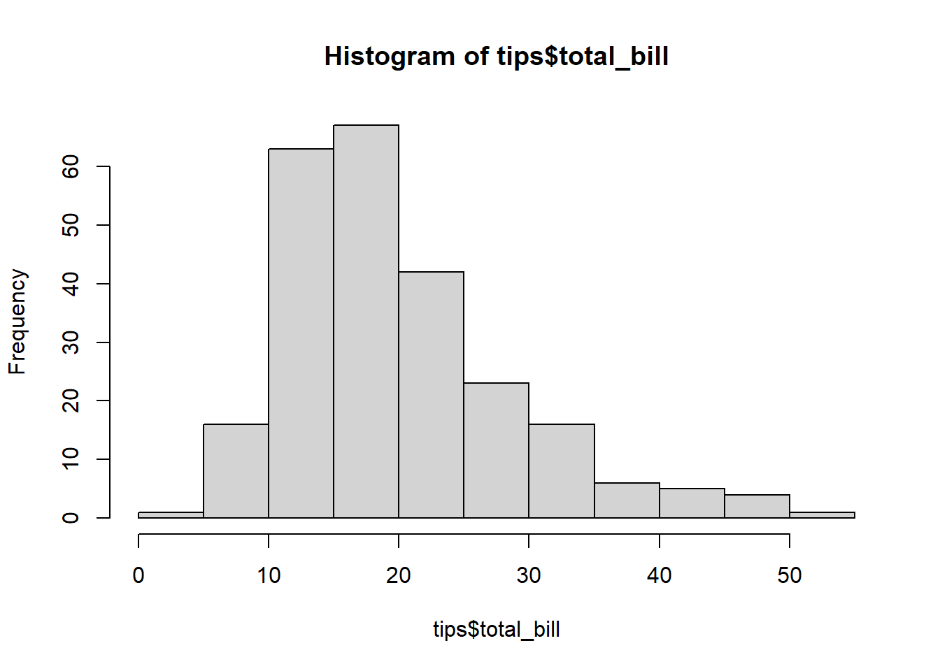
hist(tips$total_bill)

# visualization
library(dplyr)

Attaching package: 'dplyr'

The following objects are masked from 'package:stats':

    filter, lag

The following objects are masked from 'package:base':

    intersect, setdiff, setequal, union

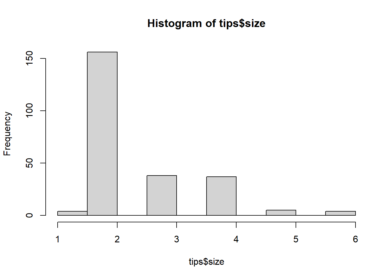
library(ggplot2)

hist(tips$size)

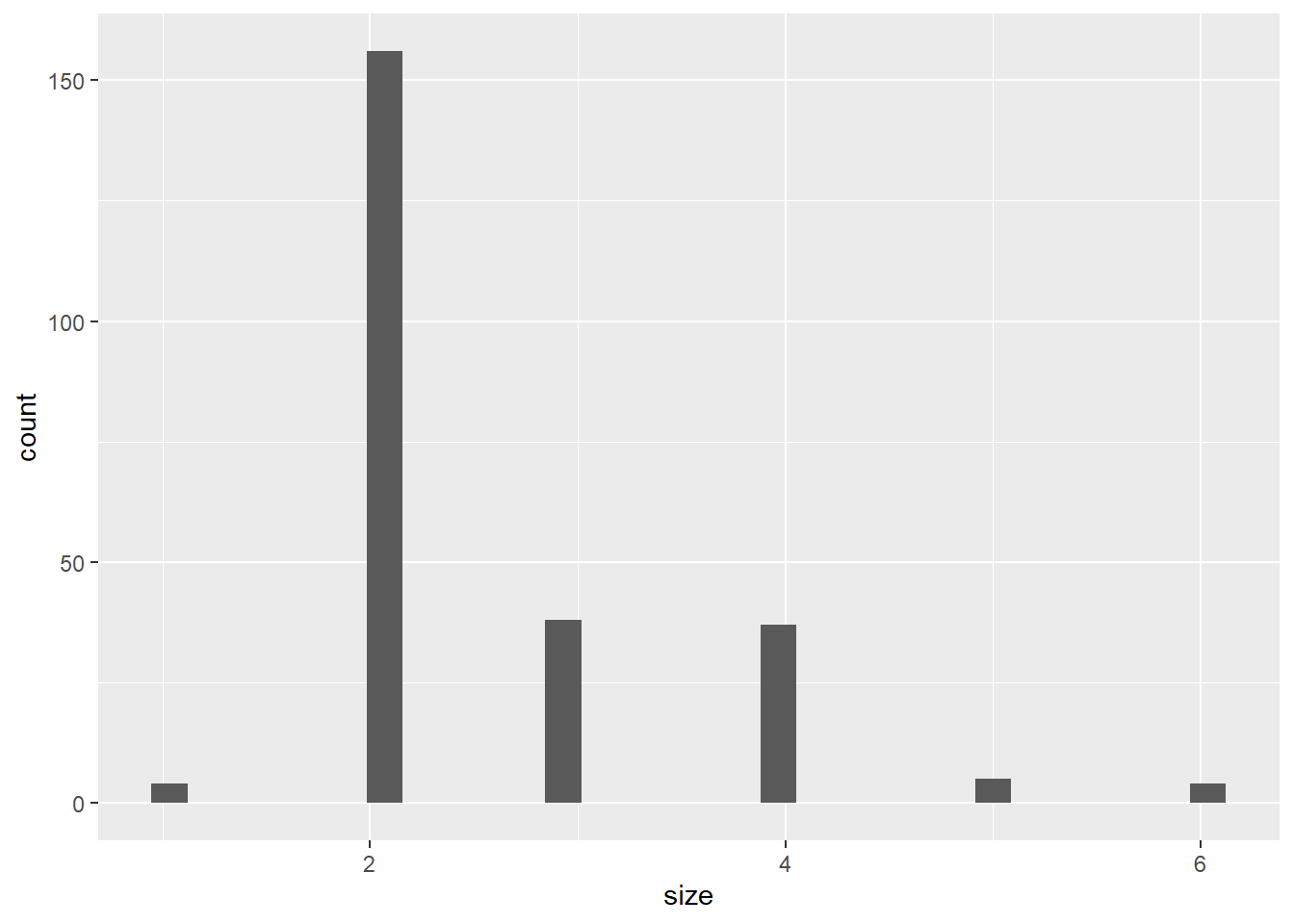
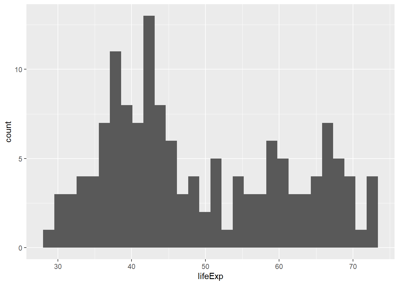
tips %>% ggplot(aes(size)) + geom_histogram()

`stat_bin()` using `bins = 30`. Pick better value with `binwidth`.

tips %>% ggplot(aes(total_bill, tip)) + geom_point()

tips %>% ggplot(aes(total_bill, tip)) + geom_point(aes(col=day))

tips %>% ggplot(aes(total_bill, tip)) + geom_point(aes(col=day, pch=sex), size=5)

tips %>% ggplot(aes(total_bill, tip)) + 
  geom_point(aes(col=day)) +
  geom_line()

tips %>% ggplot(aes(total_bill, tip, col=day, pch=sex)) + geom_point(size=3)

# 03 Data type #

x = 5
y = 2
x/y

[1] 2.5

xi = 1 + 2i
yi = 1 - 2i
xi+yi

[1] 2+0i

str = "Hello, World!"
str

[1] "Hello, World!"

blood.type = factor(c('A', 'B', 'O', 'AB'))
blood.type

[1] A  B  O  AB
Levels: A AB B O

T

[1] TRUE

F

[1] FALSE

xinf = Inf
yinf = -Inf
xinf/yinf

[1] NaN

x = 1       # x에 단순히 1을 넣은 경우 x는 숫자형
x

[1] 1

is.integer(x)

[1] FALSE

x = 1L      # x에 1L을 입력한 경우 x는 정수형
x

[1] 1

is.integer(x)

[1] TRUE

x = as.integer(1)   # x에 1을 as.integer 함수로 변환하여 입력한 경우 x는 정수형
x

[1] 1

is.integer(x)

[1] TRUE

# 05 벡터 #
1:7         # 1부터 7까지 1씩 증가시켜 요소가 7개인 벡터 생성

[1] 1 2 3 4 5 6 7

7:1         # 7부터 1까지 1씩 감소시켜 요소가 7개인 벡터 생성

[1] 7 6 5 4 3 2 1

vector(length = 5)

[1] FALSE FALSE FALSE FALSE FALSE

c(1:5)      # 1~5 요소로 구성된 벡터 생성. 1:5와 동일

[1] 1 2 3 4 5

c(1, 2, 3, c(4:6))  # 1~3 요소와 4~6 요소를 결합한 1~6 요소로 구성된 벡터 생성

[1] 1 2 3 4 5 6

x = c(1, 2, 3)  # 1~3 요소로 구성된 벡터를 x에 저장
x       # x 출력

[1] 1 2 3

y = c()         # y를 빈 벡터로 생성
y = c(y, c(1:3))    # 기존 y 벡터에 c(1:3) 벡터를 추가해 생성
y       # y 출력

[1] 1 2 3

seq(from = 1, to = 10, by = 2)  # 1부터 10까지 2씩 증가하는 벡터 생성

[1] 1 3 5 7 9

seq(1, 10, by = 2)          # 1부터 10까지 2씩 증가하는 벡터 생성

[1] 1 3 5 7 9

seq(0, 1, by = 0.1)             # 0부터 1까지 0.1씩 증가하는 요소가 11개인 벡터 생성

 [1] 0.0 0.1 0.2 0.3 0.4 0.5 0.6 0.7 0.8 0.9 1.0

seq(0, 1, length.out = 11)      # 0부터 1까지 요소가 11개인 벡터 생성

 [1] 0.0 0.1 0.2 0.3 0.4 0.5 0.6 0.7 0.8 0.9 1.0

rep(c(1:3), times = 2)      # (1, 2, 3) 벡터를 2번 반복한 벡터 생성

[1] 1 2 3 1 2 3

rep(c(1:3), each = 2)       # (1, 2, 3) 벡터의 개별 요소를 2번 반복한 벡터 생성

[1] 1 1 2 2 3 3

x = c(2, 4, 6, 8, 10)
length(x)       # x 벡터의 길이(크기)를 구함

[1] 5

x[1]        # x 벡터의 1번 요소 값을 구함

[1] 2

# x[1, 2, 3]        # x 벡터의 1, 2, 3번 요소를 구할 때 이렇게 입력하면 오류
x[c(1, 2, 3)]   # x 벡터의 1, 2, 3번 요소를 구할 때는 벡터로 묶어야 함

[1] 2 4 6

x[-c(1, 2, 3)]  # x 벡터에서 1, 2, 3번 요소를 제외한 값 출력

[1]  8 10

x[c(1:3)]       # x 벡터에서 1번부터 3번 요소를 출력

[1] 2 4 6

x = c(1, 2, 3, 4)
y = c(5, 6, 7, 8)
z = c(3, 4)
w = c(5, 6, 7)
x+2         # x 벡터의 개별 요소에 2를 각각 더함

[1] 3 4 5 6

x + y       # x 벡터와 y 벡터의 크기가 동일하므로 각 요소별로 더함

[1]  6  8 10 12

x + z       # x 벡터가 z 벡터 크기의 정수배인 경우엔 작은 쪽 벡터 요소를 순환하며 더함

[1] 4 6 6 8

x + w       # x와 w의 크기가 정수배가 아니므로 연산 오류

Warning in x + w: longer object length is not a multiple of shorter object
length

[1]  6  8 10  9

x >5        # x 벡터의 요소 값이 5보다 큰지 확인

[1] FALSE FALSE FALSE FALSE

all(x>5)        # x 벡터의 요소 값이 모두 5보다 큰지 확인

[1] FALSE

any(x>5)        # x 벡터의 요소 값 중 일부가 5보다 큰지 확인

[1] FALSE

x = 1:10
head(x)         # 데이터의 앞 6개 요소를 추출

[1] 1 2 3 4 5 6

tail(x)         # 데이터의 뒤 6개 요소를 추출

[1]  5  6  7  8  9 10

head(x, 3)  # 데이터의 앞 3개 요소를 추출

[1] 1 2 3

tail(x, 3)      # 데이터의 뒤 3개 요소를 추출

[1]  8  9 10

x = c(1, 2, 3)
y = c(3, 4, 5)
z = c(3, 1, 2)
union(x, y)     # 합집합

[1] 1 2 3 4 5

intersect(x, y)     # 교집합

[1] 3

setdiff(x, y)   # 차집합(x에서 y와 동일한 요소 제외)

[1] 1 2

setdiff(y, x)   # 차집합(y에서 x와 동일 요소 제외)

[1] 4 5

setequal(x, y)  # x와 y에 동일한 요소가 있는지 비교

[1] FALSE

setequal(x, z)  # x와 z에 동일한 요소가 있는지 비교

[1] TRUE

# 06 행렬 #
# N차원 배열 생성
x = array(1:5, c(2, 4)) # 1~5 값을 2× 4 행렬에 할당
x

     [,1] [,2] [,3] [,4]
[1,]    1    3    5    2
[2,]    2    4    1    3

x[1, ] # 1행 요소 값 출력

[1] 1 3 5 2

x[, 2] # 2열 요소 값 출력

[1] 3 4

dimnamex = list(c("1st", "2nd"), c("1st", "2nd", "3rd", "4th")) # 행과 열 이름 설정
x = array(1:5, c(2, 4), dimnames = dimnamex)
x

    1st 2nd 3rd 4th
1st   1   3   5   2
2nd   2   4   1   3

x["1st", ]

1st 2nd 3rd 4th 
  1   3   5   2 

x[, "4th"]

1st 2nd 
  2   3 

# 2차원 배열 생성
x = 1:12
x

 [1]  1  2  3  4  5  6  7  8  9 10 11 12

matrix(x, nrow = 3)

     [,1] [,2] [,3] [,4]
[1,]    1    4    7   10
[2,]    2    5    8   11
[3,]    3    6    9   12

matrix(x, nrow = 3, byrow = T)

     [,1] [,2] [,3] [,4]
[1,]    1    2    3    4
[2,]    5    6    7    8
[3,]    9   10   11   12

# 벡터를 묶어 배열 생성
v1 = c(1, 2, 3, 4)
v2 = c(5, 6, 7, 8)
v3 = c(9, 10, 11, 12)
cbind(v1, v2, v3) # 열 단위로 묶어 배열 생성

     v1 v2 v3
[1,]  1  5  9
[2,]  2  6 10
[3,]  3  7 11
[4,]  4  8 12

rbind(v1, v2, v3) # 행 단위로 묶어 배열 생성

   [,1] [,2] [,3] [,4]
v1    1    2    3    4
v2    5    6    7    8
v3    9   10   11   12

# [표 3-7]의 연산자를 활용한 다양한 행렬 연산
# 2×2 행렬 2개를 각각 x, y에 저장
x = array(1:4, dim = c(2, 2))
y = array(5:8, dim = c(2, 2))
x

     [,1] [,2]
[1,]    1    3
[2,]    2    4

y

     [,1] [,2]
[1,]    5    7
[2,]    6    8

x + y

     [,1] [,2]
[1,]    6   10
[2,]    8   12

x - y

     [,1] [,2]
[1,]   -4   -4
[2,]   -4   -4

x * y # 각 열별 곱셈

     [,1] [,2]
[1,]    5   21
[2,]   12   32

x %*% y # 수학적인 행렬 곱셈

     [,1] [,2]
[1,]   23   31
[2,]   34   46

t(x) # x의 전치 행렬

     [,1] [,2]
[1,]    1    2
[2,]    3    4

solve(x) # x의 역행렬

     [,1] [,2]
[1,]   -2  1.5
[2,]    1 -0.5

det(x) # x의 행렬식

[1] -2

x = array(1:12, c(3, 4))
x

     [,1] [,2] [,3] [,4]
[1,]    1    4    7   10
[2,]    2    5    8   11
[3,]    3    6    9   12

apply(x, 1, mean) # 가운데 값이 1이면 함수를 행별로 적용

[1] 5.5 6.5 7.5

apply(x, 2, mean) # 가운데 값이 2이면 함수를 열별로 적용

[1]  2  5  8 11

x = array(1:12, c(3, 4))
dim(x)

[1] 3 4

x = array(1:12, c(3, 4))
sample(x) # 배열 요소를 임의로 섞어 추출

 [1]  2 10 11  1  9  5  4  6  3  7 12  8

sample(x, 10) # 배열 요소 중 10개를 골라 추출

 [1] 12  6  2  4 11  5  9  3  1 10

sample(x, 10, prob = c(1:12)/24) # 각 요소별 추출 확률을 달리할 수 있음

 [1]  5  9 10  8 12 11  7  2  3  6

sample(10) # 단순히 숫자만 사용하여 샘플을 만들 수 있음

 [1]  3  6  9 10  1  7  2  4  5  8

# 07 데이터 프레임 #
name = c("철수", "춘향", "길동")
age = c(22, 20, 25)
gender = factor(c("M", "F", "M"))
blood.type = factor(c("A", "O", "B"))
patients = data.frame(name, age, gender, blood.type)
patients

  name age gender blood.type
1 철수  22      M          A
2 춘향  20      F          O
3 길동  25      M          B

# 다음과 같이 한 행으로 작성할 수도 있음
patients1 = data.frame(name = c("철수", "춘향", "길동"), age = c(22, 20, 25), gender = factor(c("M", "F", "M")), blood.type = factor(c("A", "O", "B")))
patients1

  name age gender blood.type
1 철수  22      M          A
2 춘향  20      F          O
3 길동  25      M          B

patients$name # name 속성 값 출력

[1] "철수" "춘향" "길동"

patients[1, ] # 1행 값 출력

  name age gender blood.type
1 철수  22      M          A

patients[, 2] # 2열 값 출력

[1] 22 20 25

patients[3, 1] # 3행 1열 값 출력

[1] "길동"

patients[patients$name=="철수", ] # 환자 중 철수에 대한 정보 추출

  name age gender blood.type
1 철수  22      M          A

patients[patients$name=="철수", c("name", "age")] # 철수 이름과 나이 정보만 추출

  name age
1 철수  22

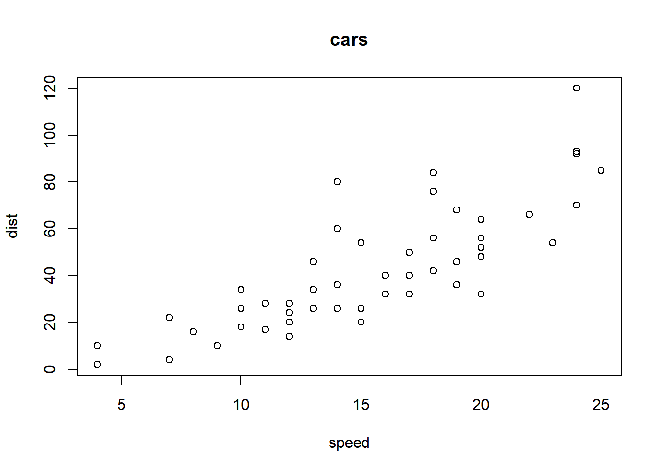
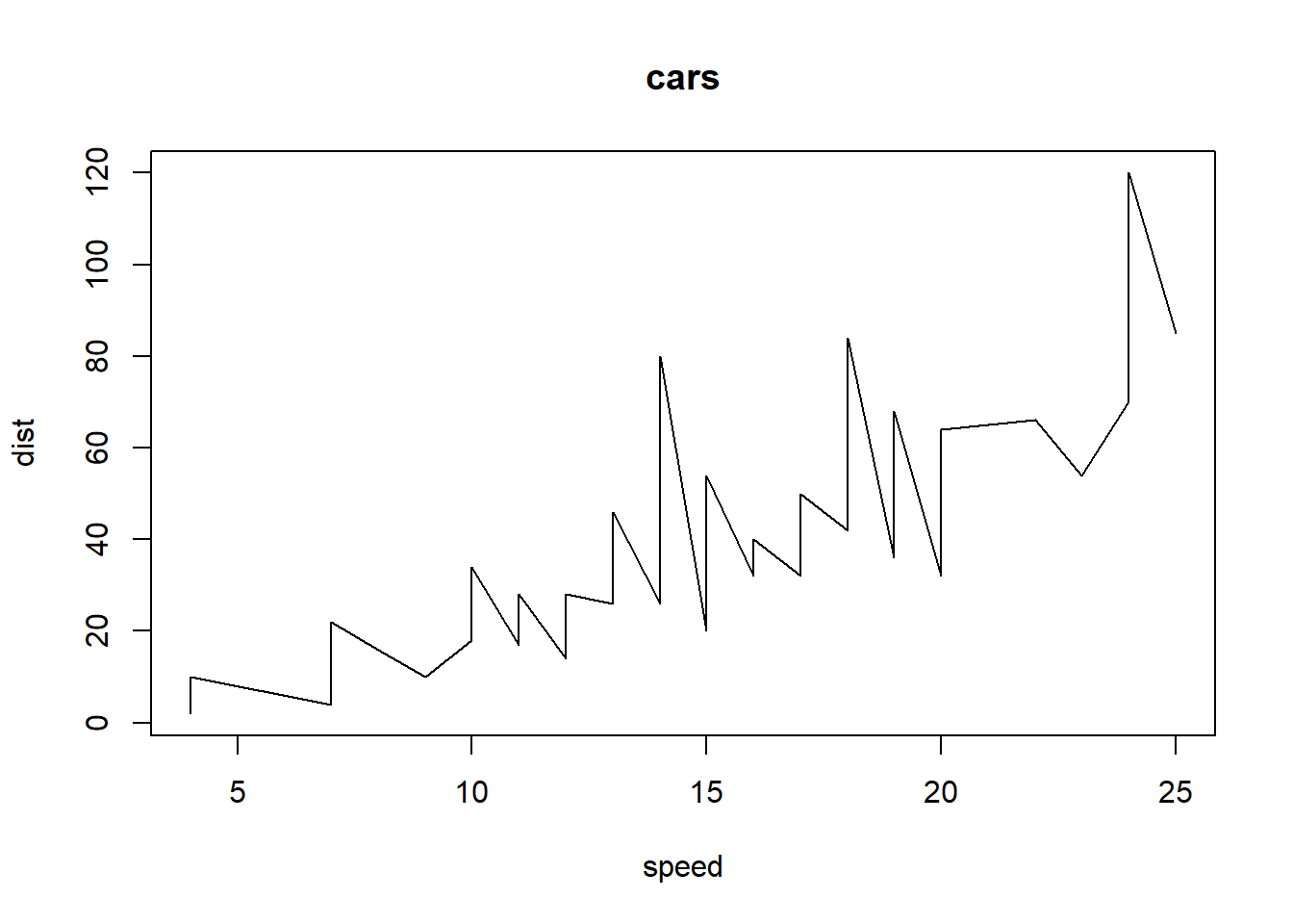
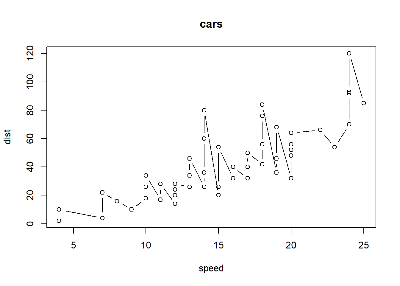
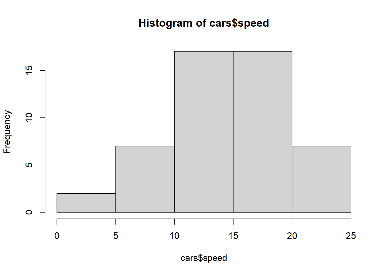
head(cars) # cars 데이터 셋 확인. head 함수의 기본 기능은 앞 6개 데이터를 추출함

  speed dist
1     4    2
2     4   10
3     7    4
4     7   22
5     8   16
6     9   10

# speed
attach(cars) # attach 함수를 통해 cars의 각 속성을 변수로 이용하게 함
# speed # speed라는 변수명을 직접 이용할 수 있음.
detach(cars) # detach 함수를 통해 cars의 각 속성을 변수로 사용하는 것을 해제함

# 데이터 속성을 이용해 함수 적용
mean(cars$speed)

[1] 15.4

max(cars$speed)

[1] 25

# with 함수를 이용해 함수 적용
with(cars, mean(speed))

[1] 15.4

with(cars, max(speed))

[1] 25

# 속도가 20 초과인 데이터만 추출
subset(cars, speed > 20)

   speed dist
44    22   66
45    23   54
46    24   70
47    24   92
48    24   93
49    24  120
50    25   85

# 속도가 20 초과인 dist 데이터만 추출, 여러 열 선택은 c( ) 안을 ,로 구분
subset(cars, speed > 20, select = c(dist))

   dist
44   66
45   54
46   70
47   92
48   93
49  120
50   85

# 속도가 20 초과인 데이터 중 dist를 제외한 데이터만 추출
subset(cars, speed > 20, select = -c(dist))

   speed
44    22
45    23
46    24
47    24
48    24
49    24
50    25

head(airquality) # airquality 데이터에는 NA가 포함되어 있음

  Ozone Solar.R Wind Temp Month Day
1    41     190  7.4   67     5   1
2    36     118  8.0   72     5   2
3    12     149 12.6   74     5   3
4    18     313 11.5   62     5   4
5    NA      NA 14.3   56     5   5
6    28      NA 14.9   66     5   6

head(na.omit(airquality)) # NA가 포함된 값을 제외하여 추출함

  Ozone Solar.R Wind Temp Month Day
1    41     190  7.4   67     5   1
2    36     118  8.0   72     5   2
3    12     149 12.6   74     5   3
4    18     313 11.5   62     5   4
7    23     299  8.6   65     5   7
8    19      99 13.8   59     5   8

# merge(x, y, by = intersect(names(x), names(y)), by.x = by, by.y = by, all = FALSE, all.x = all, all.y = all, sort = TRUE, suffixes = c(".x",".y"), incomparables = NULL, ...)

name = c("철수", "춘향", "길동")
age = c(22, 20, 25)
gender = factor(c("M", "F", "M"))
blood.type = factor(c("A", "O", "B"))
patients1 = data.frame(name, age, gender)
patients1

  name age gender
1 철수  22      M
2 춘향  20      F
3 길동  25      M

patients2 = data.frame(name, blood.type)
patients2

  name blood.type
1 철수          A
2 춘향          O
3 길동          B

patients = merge(patients1, patients2, by = "name")
patients

  name age gender blood.type
1 길동  25      M          B
2 철수  22      M          A
3 춘향  20      F          O

# 이름이 같은 열 변수가 없다면, merge 함수의 by.x와 by.y에 합칠 때
# 사용할 열의 속성명을 각각 기입해주어야 함
name1 = c("철수", "춘향", "길동")
name2 = c("민수", "춘향", "길동")
age = c(22, 20, 25)
gender = factor(c("M", "F", "M"))
blood.type = factor(c("A", "O", "B"))
patients1 = data.frame(name1, age, gender)
patients1

  name1 age gender
1  철수  22      M
2  춘향  20      F
3  길동  25      M

patients2 = data.frame(name2, blood.type)
patients2

  name2 blood.type
1  민수          A
2  춘향          O
3  길동          B

patients = merge(patients1, patients2, by.x = "name1", by.y = "name2")
patients

  name1 age gender blood.type
1  길동  25      M          B
2  춘향  20      F          O

patients = merge(patients1, patients2, by.x = "name1", by.y = "name2", all = TRUE)
patients

  name1 age gender blood.type
1  길동  25      M          B
2  민수  NA   <NA>          A
3  철수  22      M       <NA>
4  춘향  20      F          O

x = array(1:12, c(3, 4))
is.data.frame(x) # 현재 x는 데이터 프레임이 아님

[1] FALSE

as.data.frame(x)

  V1 V2 V3 V4
1  1  4  7 10
2  2  5  8 11
3  3  6  9 12

# is.data.frame 함수를 호출하는 것만으로 x가 데이터 프레임으로 바뀌지 않음
is.data.frame(x)

[1] FALSE

# as.data.frame 함수로 x를 데이터 프레임 형식으로 변환
x = as.data.frame(x)
x

  V1 V2 V3 V4
1  1  4  7 10
2  2  5  8 11
3  3  6  9 12

# x가 데이터 프레임 형식으로 변환되었음을 확인
is.data.frame(x)

[1] TRUE

# 데이터 프레임으로 변환 시 자동 지정되는 열 이름을 names 함수로 재지정함
names(x) = c("1st", "2nd", "3rd", "4th")
x

  1st 2nd 3rd 4th
1   1   4   7  10
2   2   5   8  11
3   3   6   9  12

# 08 리스트 #
patients = data.frame(name = c("철수", "춘향", "길동"), age = c(22, 20, 25), gender = factor(c("M", "F", "M")), blood.type = factor(c("A", "O", "B")))
no.patients = data.frame(day = c(1:6), no = c(50, 60, 55, 52, 65, 58))


# 데이터를 단순 추가
listPatients = list(patients, no.patients) 
listPatients

[[1]]
  name age gender blood.type
1 철수  22      M          A
2 춘향  20      F          O
3 길동  25      M          B

[[2]]
  day no
1   1 50
2   2 60
3   3 55
4   4 52
5   5 65
6   6 58

# 각 데이터에 이름을 부여하면서 추가 
listPatients = list(patients=patients, no.patients = no.patients) 
listPatients

$patients
  name age gender blood.type
1 철수  22      M          A
2 춘향  20      F          O
3 길동  25      M          B

$no.patients
  day no
1   1 50
2   2 60
3   3 55
4   4 52
5   5 65
6   6 58

listPatients$patients       # 요소명 입력

  name age gender blood.type
1 철수  22      M          A
2 춘향  20      F          O
3 길동  25      M          B

listPatients[[1]]               # 인덱스 입력

  name age gender blood.type
1 철수  22      M          A
2 춘향  20      F          O
3 길동  25      M          B

listPatients[["patients"]]          # 요소명을 ""에 입력

  name age gender blood.type
1 철수  22      M          A
2 춘향  20      F          O
3 길동  25      M          B

listPatients[["no.patients"]]       # 요소명을 ""에 입력

  day no
1   1 50
2   2 60
3   3 55
4   4 52
5   5 65
6   6 58

# no.patients 요소의 평균을 구해줌
lapply(listPatients$no.patients, mean) 

$day
[1] 3.5

$no
[1] 56.66667

# patients 요소의 평균을 구해줌. 숫자 형태가 아닌 것은 평균이 구해지지 않음
lapply(listPatients$patients, mean) 

Warning in mean.default(X[[i]], ...): argument is not numeric or logical:
returning NA

Warning in mean.default(X[[i]], ...): argument is not numeric or logical:
returning NA

Warning in mean.default(X[[i]], ...): argument is not numeric or logical:
returning NA

$name
[1] NA

$age
[1] 22.33333

$gender
[1] NA

$blood.type
[1] NA

sapply(listPatients$no.patients, mean) 

     day       no 
 3.50000 56.66667 

# sapply()의 simplify 옵션을 F로 하면 lapply() 결과와 동일한 결과를 반환함
sapply(listPatients$no.patients, mean, simplify = F) 

$day
[1] 3.5

$no
[1] 56.66667

# 01 파일 읽고 쓰기 #

# 파일 마지막 행에서 [Enter]를 누르지 않은 경우
students = read.table("data_2/students1.txt", header = T, fileEncoding = "CP949", encoding = "UTF-8")

# 파일 마지막 행에서 [Enter]를 누른 경우
students = read.table("data_2/students2.txt",  header = T, fileEncoding = "CP949", encoding = "UTF-8") 

# 읽은 파일의 구조 확인
str(students) 

'data.frame':   5 obs. of  4 variables:
 $ name   : chr  "강서준" "김도형" "박정원" "이상훈" ...
 $ korean : int  100 90 90 100 85
 $ english: int  90 100 95 85 100
 $ math   : int  100 80 90 95 100

# 파일을 있는 형태 그대로 읽음
students = read.table("data_2/students1.txt", header = T, as.is = T, fileEncoding = "CP949", encoding = "UTF-8") 
str(students)

'data.frame':   5 obs. of  4 variables:
 $ name   : chr  "강서준" "김도형" "박정원" "이상훈" ...
 $ korean : int  100 90 90 100 85
 $ english: int  90 100 95 85 100
 $ math   : int  100 80 90 95 100

# 파일을 읽을 때 문장을 요인으로 인식하지 않도록 설정
students = read.table("data_2/students1.txt", header = T, stringsAsFactors = F, fileEncoding = "CP949", encoding = "UTF-8") 
str(students)

'data.frame':   5 obs. of  4 variables:
 $ name   : chr  "강서준" "김도형" "박정원" "이상훈" ...
 $ korean : int  100 90 90 100 85
 $ english: int  90 100 95 85 100
 $ math   : int  100 80 90 95 100

# 구분 기호는 쉼표(,), 첫 행은 header로 인식하여 파일을 있는 그대로 읽어들이면 
# NA로 인해 math 요소가 문장으로 인식됨
students = read.table("data_2/students3.txt", sep = ",", header = T, as.is = T, fileEncoding = "CP949", encoding = "UTF-8") 
str(students)

'data.frame':   5 obs. of  4 variables:
 $ name   : chr  "강서준" "김도형" "박정원" "이상훈" ...
 $ korean : int  100 90 90 100 85
 $ english: int  90 100 95 85 100
 $ math   : chr  " 100" " 80" " 90" " NA" ...

# "NA" 문장을 결측값 NA로 처리하라고 해도 처리가 안됨. 정확한 문장은 NA 앞에 빈 칸이 있어야 하기 때문
students = read.table("data_2/students3.txt", sep = ",", header = T, as.is = T, na.strings = "NA", fileEncoding = "CP949", encoding = "UTF-8")  
str(students)

'data.frame':   5 obs. of  4 variables:
 $ name   : chr  "강서준" "김도형" "박정원" "이상훈" ...
 $ korean : int  100 90 90 100 85
 $ english: int  90 100 95 85 100
 $ math   : chr  " 100" " 80" " 90" " NA" ...

# "NA"로 정확하게 입력하자 결측값 NA로 처리되면서 math 요소가 모두 숫자로 인식됨
students = read.table("data_2/students3.txt", sep = ",", header = T, as.is = T, na.strings = " NA", fileEncoding = "CP949", encoding = "UTF-8") 
str(students)

'data.frame':   5 obs. of  4 variables:
 $ name   : chr  "강서준" "김도형" "박정원" "이상훈" ...
 $ korean : int  100 90 90 100 85
 $ english: int  90 100 95 85 100
 $ math   : int  100 80 90 NA 100

# strip.white에서 빈칸을 제거하면 na.string의 기본값이 "NA"로 설정되어 math 요소가 모두 숫자로 인식됨.
students = read.table("data_2/students3.txt", sep = ",", header = T, as.is = T, strip.white = T, fileEncoding = "CP949", encoding = "UTF-8") 
str(students)

'data.frame':   5 obs. of  4 variables:
 $ name   : chr  "강서준" "김도형" "박정원" "이상훈" ...
 $ korean : int  100 90 90 100 85
 $ english: int  90 100 95 85 100
 $ math   : int  100 80 90 NA 100

# 첫 행이 header이므로 header 옵션을 지정할 필요가 없음
students = read.csv("data_2/students.csv", fileEncoding = "CP949", encoding = "UTF-8") 
students

    name korean english math
1 강서준    100      90  100
2 김도형     90     100   80
3 박정원     90      95   90
4 이상훈    100      85   95
5 최건우     85     100  100

# 읽은 파일의 구조 확인
str(students) 

'data.frame':   5 obs. of  4 variables:
 $ name   : chr  "강서준" "김도형" "박정원" "이상훈" ...
 $ korean : int  100 90 90 100 85
 $ english: int  90 100 95 85 100
 $ math   : int  100 80 90 95 100

# name 속성을 요인에서 문장으로 변경
students$name = as.character(students$name) 
str(students)

'data.frame':   5 obs. of  4 variables:
 $ name   : chr  "강서준" "김도형" "박정원" "이상훈" ...
 $ korean : int  100 90 90 100 85
 $ english: int  90 100 95 85 100
 $ math   : int  100 80 90 95 100

# 파일을 읽을 때 문장을 요인으로 인식하지 않도록 설정함
students = read.csv("data_2/students.csv", stringsAsFactors = FALSE, fileEncoding = "CP949", encoding = "UTF-8") 
str(students)

'data.frame':   5 obs. of  4 variables:
 $ name   : chr  "강서준" "김도형" "박정원" "이상훈" ...
 $ korean : int  100 90 90 100 85
 $ english: int  90 100 95 85 100
 $ math   : int  100 80 90 95 100

# 문장에 큰따옴표가 표시됨.
write.table(students, file = "data_2/output.txt") 

# 문장에 큰따옴표되지 않음.
write.table(students, file = "data_2/output.txt", quote = F) 

# 02 데이터 정제를 위한 조건문과 반복문 #

test = c(15, 20, 30, NA, 45)    # 벡터인 경우
test[test<40]   # 값이 40 미만인 요소 추출

[1] 15 20 30 NA

test[test%%3!= 0]   # 값이 3으로 나누어 떨어지지 않는 요소 추출

[1] 20 NA

test[is.na(test)]   # NA인 요소 추출

[1] NA

test[!is.na(test)]          # NA가 아닌 요소 추출

[1] 15 20 30 45

test[test%%2==0 & !is.na(test)] # 2의 배수면서 NA가 아닌 요소 추출

[1] 20 30

characters = data.frame(name = c("길동", "춘향", "철수"), 
                        age = c(30, 16, 21), 
                        gender = factor(c("M", "F","M")))  
# 데이터 프레임인 경우

characters

  name age gender
1 길동  30      M
2 춘향  16      F
3 철수  21      M

characters[characters$gender =="F",1]  # 성별이 여성인 행 추출

[1] "춘향"

library(dplyr)

characters %>% filter(gender=="F") %>% select(name)

  name
1 춘향

characters[characters$age<30 & characters$gender =="M",] 

  name age gender
3 철수  21      M

# 30살 미만의 남성 행 추출                    
characters %>% filter(age<30 & gender=="M")

  name age gender
1 철수  21      M

x = 5
if(x %% 2 ==0) {
  print('x는 짝수')    # 조건식이 참일 때 수행
}   else {
  print('x는 홀수')    # 조건식이 거짓일 때 수행
}

[1] "x는 홀수"

x = 8
if(x>0) {
  print('x is a positive value.')   # x가 0보다 크면 출력
} else if(x<0) {
  print('x is a negative value.')   # 위 조건을 만족하지 않고 x가 0보다 작으면 출력
} else {
  print('x is zero.')       # 위 조건을 모두 만족하지 않으면 출력
}

[1] "x is a positive value."

x = c(-5:5)
options(digits = 3)     # 숫자 표현 시 유효자릿수를 3자리로 설정
sqrt(x)

Warning in sqrt(x): NaNs produced

 [1]  NaN  NaN  NaN  NaN  NaN 0.00 1.00 1.41 1.73 2.00 2.24

sqrt(ifelse(x>=0, x, NA))   # NaN이 발생하지 않게 음수면 NA로 표시

 [1]   NA   NA   NA   NA   NA 0.00 1.00 1.41 1.73 2.00 2.24

students = read.csv("data_2/students2.csv", fileEncoding = "CP949", encoding = "UTF-8")
students         # 데이터에 100 초과 값과 음수 값이 포함되어 있음.

    name korean english math
1 강서준    100      90  100
2 김도형     90     120   80
3 박정원     90      95   90
4 이상훈    100      85 -100
5 최건우     85     100  100

students[, 2] = ifelse(students[, 2]>= 0 & students[, 2]<= 100, 
                       students[, 2], NA)
students[, 3] = ifelse(students[, 3]>= 0 & students[, 3]<= 100, 
                       students[, 3], NA)
students[, 4] = ifelse(students[, 4]>= 0 & students[, 4]<= 100, 
                       students[, 4], NA)
students         # ifelse 문으로 2~4열 값 중 0~100 외의 값은 NA로 처리함.

    name korean english math
1 강서준    100      90  100
2 김도형     90      NA   80
3 박정원     90      95   90
4 이상훈    100      85   NA
5 최건우     85     100  100

# repeat 문을 이용해 1부터 10까지 숫자 증가시키기
i = 1                # i의 시작값은 1
repeat {
  if(i>10) {         # i가 10을 넘으면 반복을 중단(break)함
    break
  } else {
    print(i)
    i = i+1           # i를 1 증가시킴.
  }
}

[1] 1
[1] 2
[1] 3
[1] 4
[1] 5
[1] 6
[1] 7
[1] 8
[1] 9
[1] 10

# while 문을 이용해 1부터 10까지 숫자 증가시키기
i = 1 # i의 시작값은 1임.
while(i < 10){ # i가 10 이하인 동안에 반복함
  print(i)
  i = i+1 # i를 1 증가시킴.
}

[1] 1
[1] 2
[1] 3
[1] 4
[1] 5
[1] 6
[1] 7
[1] 8
[1] 9

# while 문을 이용해 구구단 2단 만들기
i = 1
while(i<10) {
  print(paste(2, "X", i, "=", 2*i))
  i = i+1
}

[1] "2 X 1 = 2"
[1] "2 X 2 = 4"
[1] "2 X 3 = 6"
[1] "2 X 4 = 8"
[1] "2 X 5 = 10"
[1] "2 X 6 = 12"
[1] "2 X 7 = 14"
[1] "2 X 8 = 16"
[1] "2 X 9 = 18"

# for 문을 이용한 1부터 10까지 숫자 증가시키기
for(i in 1:10) {
  print(i)
}  

[1] 1
[1] 2
[1] 3
[1] 4
[1] 5
[1] 6
[1] 7
[1] 8
[1] 9
[1] 10

# for 문을 이용해 구구단 2단 만들기
for(i in 1:9) {
  print(paste(2, "X", i, "=", 2*i))
}

[1] "2 X 1 = 2"
[1] "2 X 2 = 4"
[1] "2 X 3 = 6"
[1] "2 X 4 = 8"
[1] "2 X 5 = 10"
[1] "2 X 6 = 12"
[1] "2 X 7 = 14"
[1] "2 X 8 = 16"
[1] "2 X 9 = 18"

# for 문을 이용해 구구단 2~9단 만들기
for(i in 2:9) {
  for(j in 1:9) {
    print(paste(i, "X", j, "=", i*j))
  }
}

[1] "2 X 1 = 2"
[1] "2 X 2 = 4"
[1] "2 X 3 = 6"
[1] "2 X 4 = 8"
[1] "2 X 5 = 10"
[1] "2 X 6 = 12"
[1] "2 X 7 = 14"
[1] "2 X 8 = 16"
[1] "2 X 9 = 18"
[1] "3 X 1 = 3"
[1] "3 X 2 = 6"
[1] "3 X 3 = 9"
[1] "3 X 4 = 12"
[1] "3 X 5 = 15"
[1] "3 X 6 = 18"
[1] "3 X 7 = 21"
[1] "3 X 8 = 24"
[1] "3 X 9 = 27"
[1] "4 X 1 = 4"
[1] "4 X 2 = 8"
[1] "4 X 3 = 12"
[1] "4 X 4 = 16"
[1] "4 X 5 = 20"
[1] "4 X 6 = 24"
[1] "4 X 7 = 28"
[1] "4 X 8 = 32"
[1] "4 X 9 = 36"
[1] "5 X 1 = 5"
[1] "5 X 2 = 10"
[1] "5 X 3 = 15"
[1] "5 X 4 = 20"
[1] "5 X 5 = 25"
[1] "5 X 6 = 30"
[1] "5 X 7 = 35"
[1] "5 X 8 = 40"
[1] "5 X 9 = 45"
[1] "6 X 1 = 6"
[1] "6 X 2 = 12"
[1] "6 X 3 = 18"
[1] "6 X 4 = 24"
[1] "6 X 5 = 30"
[1] "6 X 6 = 36"
[1] "6 X 7 = 42"
[1] "6 X 8 = 48"
[1] "6 X 9 = 54"
[1] "7 X 1 = 7"
[1] "7 X 2 = 14"
[1] "7 X 3 = 21"
[1] "7 X 4 = 28"
[1] "7 X 5 = 35"
[1] "7 X 6 = 42"
[1] "7 X 7 = 49"
[1] "7 X 8 = 56"
[1] "7 X 9 = 63"
[1] "8 X 1 = 8"
[1] "8 X 2 = 16"
[1] "8 X 3 = 24"
[1] "8 X 4 = 32"
[1] "8 X 5 = 40"
[1] "8 X 6 = 48"
[1] "8 X 7 = 56"
[1] "8 X 8 = 64"
[1] "8 X 9 = 72"
[1] "9 X 1 = 9"
[1] "9 X 2 = 18"
[1] "9 X 3 = 27"
[1] "9 X 4 = 36"
[1] "9 X 5 = 45"
[1] "9 X 6 = 54"
[1] "9 X 7 = 63"
[1] "9 X 8 = 72"
[1] "9 X 9 = 81"

# 1부터 10까지의 수 중 짝수만 출력하기
for(i in 1:10) {
  if(i%%2 == 0) {
    print(i)
  }
}

[1] 2
[1] 4
[1] 6
[1] 8
[1] 10

# 1부터 10까지의 수 중 소수 출력하기
for(i in 1:10) {
  check = 0
  for(j in 1:i) {
    if(i%%j ==0) {
      check = check+1
    }
  }
  if(check ==2) { 
    print(i)
  }
}

[1] 2
[1] 3
[1] 5
[1] 7

students = read.csv("data_2/students2.csv", fileEncoding = "CP949", encoding = "UTF-8")
students        # 데이터에 100 초과 값과 음수 값이 포함되어 있음

    name korean english math
1 강서준    100      90  100
2 김도형     90     120   80
3 박정원     90      95   90
4 이상훈    100      85 -100
5 최건우     85     100  100

for(i in 2:4) {
  students[, i] = ifelse(students[, i]>= 0 & students[, i]<= 100, 
                         students[, i], NA)
}


students        # ifelse 문으로 2~4열 값 중 0~100 외의 값은 NA로 처리함

    name korean english math
1 강서준    100      90  100
2 김도형     90      NA   80
3 박정원     90      95   90
4 이상훈    100      85   NA
5 최건우     85     100  100

# 03 사용자 정의 함수 : 원하는 기능 묶기 # 
x=5
fa = 1  # 계승값을 저장할 변수
while(x>1) {  # x가 1보다 큰 동안 반복
  
  fa = fa*x   # x 값을 fa에 곱한 후 fa에 다시 저장
  x = x-1  # x 값을 1 감소
  x
}  
fa

[1] 120

fact = function(x) {   # 함수의 이름은 fact, 입력은 x
  fa = 1  # 계승값을 저장할 변수
  while(x>1) {  # x가 1보다 큰 동안 반복
    fa = fa*x   # x 값을 fa에 곱한 후 fa에 다시 저장
    x = x-1  # x 값을 1 감소
  }  
  return(fa)   # 최종 계산된 fa 반환
}
fact(5)   # 5!을 계산한 결과 출력

[1] 120

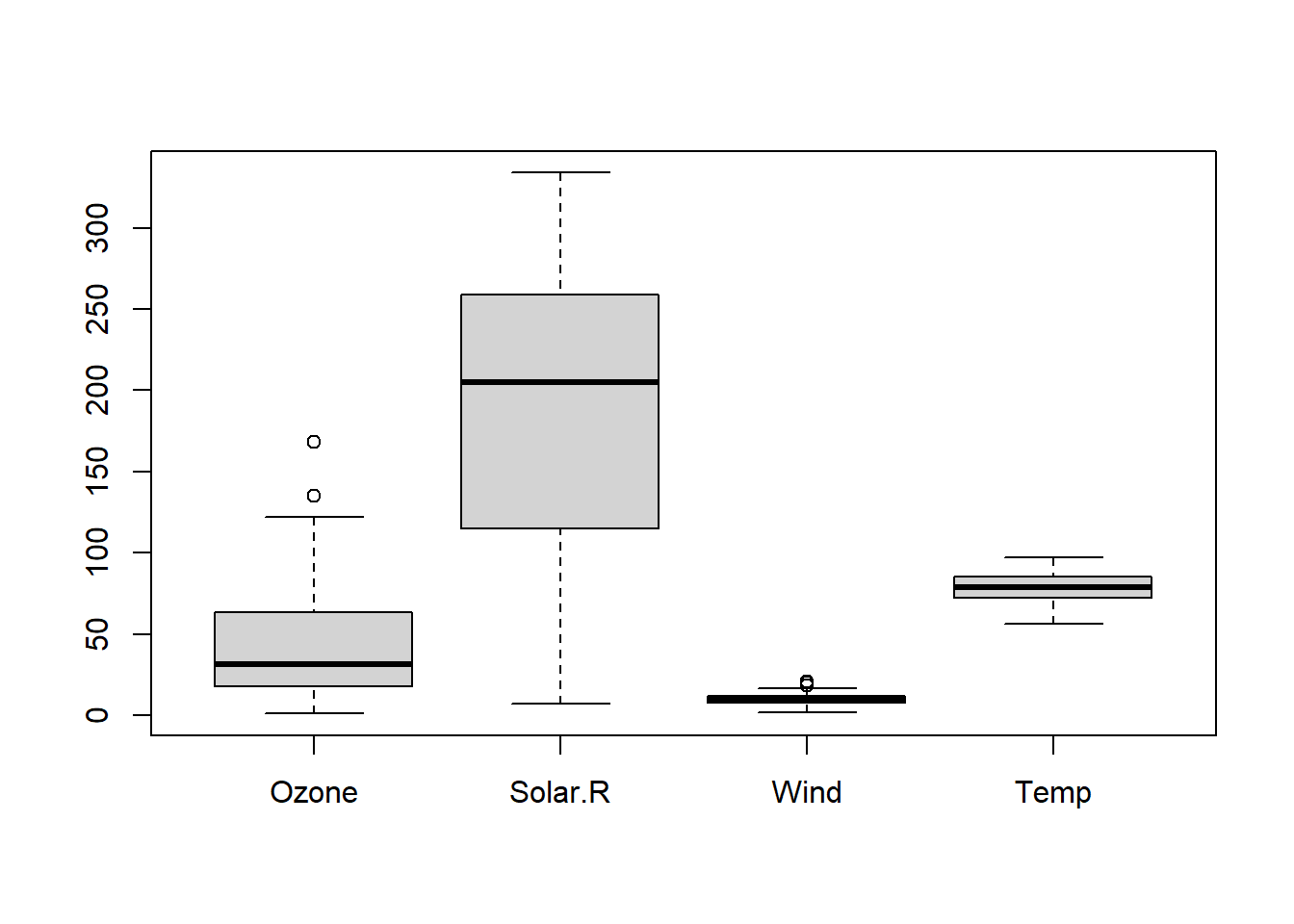
my.is.na<-function(x) { # table(is.na()) 함수를 하나로 묶은 my.is.na 함수를 만듦
  table(is.na(x))
}

my.is.na(airquality)    # 이 결과는 table(is.na(airquality))와 같음.

FALSE  TRUE 
  874    44 

table(is.na(airquality))

FALSE  TRUE 
  874    44 

# 04 데이터 정제 예제 1 : 결측값 처리 # 

# is.na 함수를 이용해 결측값 처리하기
str(airquality) # airquality 데이터의 구조를 살펴봄.

'data.frame':   153 obs. of  6 variables:
 $ Ozone  : int  41 36 12 18 NA 28 23 19 8 NA ...
 $ Solar.R: int  190 118 149 313 NA NA 299 99 19 194 ...
 $ Wind   : num  7.4 8 12.6 11.5 14.3 14.9 8.6 13.8 20.1 8.6 ...
 $ Temp   : int  67 72 74 62 56 66 65 59 61 69 ...
 $ Month  : int  5 5 5 5 5 5 5 5 5 5 ...
 $ Day    : int  1 2 3 4 5 6 7 8 9 10 ...

# airquality 데이터에서 NA인 것은 TRUE, 아니면 FALSE로 나타냄. 데이터가 많아 head 함수로 추려냄.
head(airquality)

  Ozone Solar.R Wind Temp Month Day
1    41     190  7.4   67     5   1
2    36     118  8.0   72     5   2
3    12     149 12.6   74     5   3
4    18     313 11.5   62     5   4
5    NA      NA 14.3   56     5   5
6    28      NA 14.9   66     5   6

head(is.na(airquality)) 

     Ozone Solar.R  Wind  Temp Month   Day
[1,] FALSE   FALSE FALSE FALSE FALSE FALSE
[2,] FALSE   FALSE FALSE FALSE FALSE FALSE
[3,] FALSE   FALSE FALSE FALSE FALSE FALSE
[4,] FALSE   FALSE FALSE FALSE FALSE FALSE
[5,]  TRUE    TRUE FALSE FALSE FALSE FALSE
[6,] FALSE    TRUE FALSE FALSE FALSE FALSE

table(is.na(airquality))    # NA가 총 44개 있음.

FALSE  TRUE 
  874    44 

sum(is.na(airquality))  # NA가 총 44개 있음.

[1] 44

table(is.na(airquality$Temp))   # Temp에는 NA가 없음을 확인함.

FALSE 
  153 

table(is.na(airquality$Ozone))  # Ozone에는 NA가 37개 발견됨.

FALSE  TRUE 
  116    37 

mean(airquality$Temp)       # NA가 없는 Temp는 평균이 구해짐.

[1] 77.9

mean(airquality$Ozone)      # NA가 있는 Ozone은 평균이 NA로 나옴.

[1] NA

air_narm = airquality[!is.na(airquality$Ozone), ] # Ozone 속성에서 NA가 없는 값만 추출함. 
air_narm

    Ozone Solar.R Wind Temp Month Day
1      41     190  7.4   67     5   1
2      36     118  8.0   72     5   2
3      12     149 12.6   74     5   3
4      18     313 11.5   62     5   4
6      28      NA 14.9   66     5   6
7      23     299  8.6   65     5   7
8      19      99 13.8   59     5   8
9       8      19 20.1   61     5   9
11      7      NA  6.9   74     5  11
12     16     256  9.7   69     5  12
13     11     290  9.2   66     5  13
14     14     274 10.9   68     5  14
15     18      65 13.2   58     5  15
16     14     334 11.5   64     5  16
17     34     307 12.0   66     5  17
18      6      78 18.4   57     5  18
19     30     322 11.5   68     5  19
20     11      44  9.7   62     5  20
21      1       8  9.7   59     5  21
22     11     320 16.6   73     5  22
23      4      25  9.7   61     5  23
24     32      92 12.0   61     5  24
28     23      13 12.0   67     5  28
29     45     252 14.9   81     5  29
30    115     223  5.7   79     5  30
31     37     279  7.4   76     5  31
38     29     127  9.7   82     6   7
40     71     291 13.8   90     6   9
41     39     323 11.5   87     6  10
44     23     148  8.0   82     6  13
47     21     191 14.9   77     6  16
48     37     284 20.7   72     6  17
49     20      37  9.2   65     6  18
50     12     120 11.5   73     6  19
51     13     137 10.3   76     6  20
62    135     269  4.1   84     7   1
63     49     248  9.2   85     7   2
64     32     236  9.2   81     7   3
66     64     175  4.6   83     7   5
67     40     314 10.9   83     7   6
68     77     276  5.1   88     7   7
69     97     267  6.3   92     7   8
70     97     272  5.7   92     7   9
71     85     175  7.4   89     7  10
73     10     264 14.3   73     7  12
74     27     175 14.9   81     7  13
76      7      48 14.3   80     7  15
77     48     260  6.9   81     7  16
78     35     274 10.3   82     7  17
79     61     285  6.3   84     7  18
80     79     187  5.1   87     7  19
81     63     220 11.5   85     7  20
82     16       7  6.9   74     7  21
85     80     294  8.6   86     7  24
86    108     223  8.0   85     7  25
87     20      81  8.6   82     7  26
88     52      82 12.0   86     7  27
89     82     213  7.4   88     7  28
90     50     275  7.4   86     7  29
91     64     253  7.4   83     7  30
92     59     254  9.2   81     7  31
93     39      83  6.9   81     8   1
94      9      24 13.8   81     8   2
95     16      77  7.4   82     8   3
96     78      NA  6.9   86     8   4
97     35      NA  7.4   85     8   5
98     66      NA  4.6   87     8   6
99    122     255  4.0   89     8   7
100    89     229 10.3   90     8   8
101   110     207  8.0   90     8   9
104    44     192 11.5   86     8  12
105    28     273 11.5   82     8  13
106    65     157  9.7   80     8  14
108    22      71 10.3   77     8  16
109    59      51  6.3   79     8  17
110    23     115  7.4   76     8  18
111    31     244 10.9   78     8  19
112    44     190 10.3   78     8  20
113    21     259 15.5   77     8  21
114     9      36 14.3   72     8  22
116    45     212  9.7   79     8  24
117   168     238  3.4   81     8  25
118    73     215  8.0   86     8  26
120    76     203  9.7   97     8  28
121   118     225  2.3   94     8  29
122    84     237  6.3   96     8  30
123    85     188  6.3   94     8  31
124    96     167  6.9   91     9   1
125    78     197  5.1   92     9   2
126    73     183  2.8   93     9   3
127    91     189  4.6   93     9   4
128    47      95  7.4   87     9   5
129    32      92 15.5   84     9   6
130    20     252 10.9   80     9   7
131    23     220 10.3   78     9   8
132    21     230 10.9   75     9   9
133    24     259  9.7   73     9  10
134    44     236 14.9   81     9  11
135    21     259 15.5   76     9  12
136    28     238  6.3   77     9  13
137     9      24 10.9   71     9  14
138    13     112 11.5   71     9  15
139    46     237  6.9   78     9  16
140    18     224 13.8   67     9  17
141    13      27 10.3   76     9  18
142    24     238 10.3   68     9  19
143    16     201  8.0   82     9  20
144    13     238 12.6   64     9  21
145    23      14  9.2   71     9  22
146    36     139 10.3   81     9  23
147     7      49 10.3   69     9  24
148    14      20 16.6   63     9  25
149    30     193  6.9   70     9  26
151    14     191 14.3   75     9  28
152    18     131  8.0   76     9  29
153    20     223 11.5   68     9  30

mean(air_narm$Ozone)    # 결측값이 제거된 데이터에서는 mean 함수가 정상적으로 동작함.

[1] 42.1

# na.omit 함수를 이용해 결측값 처리하기
air_narm1 = na.omit(airquality)
mean(air_narm1$Ozone)

[1] 42.1

# 함수 속성인 na.rm을 이용해 결측값 처리하기
mean(airquality$Ozone, na.rm = T)

[1] 42.1

mean(airquality$Ozone, na.rm = F)

[1] NA

table(is.na(airquality))

FALSE  TRUE 
  874    44 

table(is.na(airquality$Ozone))

FALSE  TRUE 
  116    37 

table(is.na(airquality$Solar.R))

FALSE  TRUE 
  146     7 

air_narm = airquality[!is.na(airquality$Ozone) & !is.na(airquality$Solar.R), ]
mean(air_narm$Ozone)

[1] 42.1

# 05 데이터 정제 예제 2 : 이상값 처리 # 

# 이상값이 포함된 환자 데이터
patients = data.frame(name = c("환자1", "환자2", "환자3", "환자4", "환자5"), age = c(22, 20, 25, 30, 27), gender=factor(c("M", "F", "M", "K", "F")), blood.type = factor(c("A", "O", "B", "AB", "C")))
patients

   name age gender blood.type
1 환자1  22      M          A
2 환자2  20      F          O
3 환자3  25      M          B
4 환자4  30      K         AB
5 환자5  27      F          C

# 성별에서 이상값 제거
patients_outrm = patients[patients$gender=="M"|patients$gender=="F", ]
patients_outrm  

   name age gender blood.type
1 환자1  22      M          A
2 환자2  20      F          O
3 환자3  25      M          B
5 환자5  27      F          C

# 성별과 혈액형에서 이상값 제거
patients_outrm1 = patients[(patients$gender == "M"|patients$gender == "F") & 
                             (patients$blood.type == "A"|
                                patients$blood.type == "B"|
                                patients$blood.type == "O"|
                                patients$blood.type == "AB"), ]
patients_outrm1  

   name age gender blood.type
1 환자1  22      M          A
2 환자2  20      F          O
3 환자3  25      M          B

# 이상값이 포함된 환자 데이터
patients = data.frame(name = c("환자1", "환자2", "환자3", "환자4", "환자5"), 
                      age = c(22, 20, 25, 30, 27), 
                      gender = c(1, 2, 1, 3, 2), 
                      blood.type = c(1, 3, 2, 4, 5))
patients    

   name age gender blood.type
1 환자1  22      1          1
2 환자2  20      2          3
3 환자3  25      1          2
4 환자4  30      3          4
5 환자5  27      2          5

# 성별에 있는 이상값을 결측값으로 변경
patients$gender = ifelse((patients$gender<1|patients$gender>2), NA, patients$gender)
patients    

   name age gender blood.type
1 환자1  22      1          1
2 환자2  20      2          3
3 환자3  25      1          2
4 환자4  30     NA          4
5 환자5  27      2          5

# 형액형에 있는 이상값도 결측값으로 변경
patients$blood.type = ifelse((patients$blood.type<1|patients$blood.type>4), NA, 
                             patients$blood.type)
patients

   name age gender blood.type
1 환자1  22      1          1
2 환자2  20      2          3
3 환자3  25      1          2
4 환자4  30     NA          4
5 환자5  27      2         NA

# 결측값을 모두 제거
patients[!is.na(patients$gender)&!is.na(patients$blood.type), ]

   name age gender blood.type
1 환자1  22      1          1
2 환자2  20      2          3
3 환자3  25      1          2

boxplot(airquality[, c(1:4)])    # Ozone, Solar.R, Wind, Temp에 대한 boxplot

boxplot(airquality[, 1])$stats   # Ozone의 boxplot 통계값 계산

      [,1]
[1,]   1.0
[2,]  18.0
[3,]  31.5
[4,]  63.5
[5,] 122.0

air = airquality                 # 임시 저장 변수로 airquality 데이터 복사
table(is.na(air$Ozone))          # Ozone의 현재 NA 개수 확인

FALSE  TRUE 
  116    37 

# 이상값을 NA로 변경
air$Ozone = ifelse(air$Ozone<1|air$Ozone>122, NA, air$Ozone) 
table(is.na(air$Ozone)) # 이상값 처리 후 NA 개수 확인(2개 증가)

FALSE  TRUE 
  114    39 

# NA 제거
air_narm = air[!is.na(air$Ozone), ] 
mean(air_narm$Ozone) # 이상값 두 개 제거로 is.na 함수를 이용한 결과보다 값이 줄어듦

[1] 40.2

# 02 베이스 R을 이용한 데이터 가공 # 

library(gapminder) 
library(dplyr)
glimpse(gapminder)

Rows: 1,704
Columns: 6
$ country   <fct> "Afghanistan", "Afghanistan", "Afghanistan", "Afghanistan", …
$ continent <fct> Asia, Asia, Asia, Asia, Asia, Asia, Asia, Asia, Asia, Asia, …
$ year      <int> 1952, 1957, 1962, 1967, 1972, 1977, 1982, 1987, 1992, 1997, …
$ lifeExp   <dbl> 28.8, 30.3, 32.0, 34.0, 36.1, 38.4, 39.9, 40.8, 41.7, 41.8, …
$ pop       <int> 8425333, 9240934, 10267083, 11537966, 13079460, 14880372, 12…
$ gdpPercap <dbl> 779, 821, 853, 836, 740, 786, 978, 852, 649, 635, 727, 975, …

gapminder[, c("country", "lifeExp")]

# A tibble: 1,704 × 2
   country     lifeExp
   <fct>         <dbl>
 1 Afghanistan    28.8
 2 Afghanistan    30.3
 3 Afghanistan    32.0
 4 Afghanistan    34.0
 5 Afghanistan    36.1
 6 Afghanistan    38.4
 7 Afghanistan    39.9
 8 Afghanistan    40.8
 9 Afghanistan    41.7
10 Afghanistan    41.8
# ℹ 1,694 more rows

gapminder[, c("country", "lifeExp", "year")]

# A tibble: 1,704 × 3
   country     lifeExp  year
   <fct>         <dbl> <int>
 1 Afghanistan    28.8  1952
 2 Afghanistan    30.3  1957
 3 Afghanistan    32.0  1962
 4 Afghanistan    34.0  1967
 5 Afghanistan    36.1  1972
 6 Afghanistan    38.4  1977
 7 Afghanistan    39.9  1982
 8 Afghanistan    40.8  1987
 9 Afghanistan    41.7  1992
10 Afghanistan    41.8  1997
# ℹ 1,694 more rows

gapminder[1:15, ]

# A tibble: 15 × 6
   country     continent  year lifeExp      pop gdpPercap
   <fct>       <fct>     <int>   <dbl>    <int>     <dbl>
 1 Afghanistan Asia       1952    28.8  8425333      779.
 2 Afghanistan Asia       1957    30.3  9240934      821.
 3 Afghanistan Asia       1962    32.0 10267083      853.
 4 Afghanistan Asia       1967    34.0 11537966      836.
 5 Afghanistan Asia       1972    36.1 13079460      740.
 6 Afghanistan Asia       1977    38.4 14880372      786.
 7 Afghanistan Asia       1982    39.9 12881816      978.
 8 Afghanistan Asia       1987    40.8 13867957      852.
 9 Afghanistan Asia       1992    41.7 16317921      649.
10 Afghanistan Asia       1997    41.8 22227415      635.
11 Afghanistan Asia       2002    42.1 25268405      727.
12 Afghanistan Asia       2007    43.8 31889923      975.
13 Albania     Europe     1952    55.2  1282697     1601.
14 Albania     Europe     1957    59.3  1476505     1942.
15 Albania     Europe     1962    64.8  1728137     2313.

library(dplyr)
gapminder %>% filter(country=="Croatia") %>% select(year, gdpPercap) %>% plot

gapminder[gapminder$country == "Croatia", ]

# A tibble: 12 × 6
   country continent  year lifeExp     pop gdpPercap
   <fct>   <fct>     <int>   <dbl>   <int>     <dbl>
 1 Croatia Europe     1952    61.2 3882229     3119.
 2 Croatia Europe     1957    64.8 3991242     4338.
 3 Croatia Europe     1962    67.1 4076557     5478.
 4 Croatia Europe     1967    68.5 4174366     6960.
 5 Croatia Europe     1972    69.6 4225310     9164.
 6 Croatia Europe     1977    70.6 4318673    11305.
 7 Croatia Europe     1982    70.5 4413368    13222.
 8 Croatia Europe     1987    71.5 4484310    13823.
 9 Croatia Europe     1992    72.5 4494013     8448.
10 Croatia Europe     1997    73.7 4444595     9876.
11 Croatia Europe     2002    74.9 4481020    11628.
12 Croatia Europe     2007    75.7 4493312    14619.

gapminder[gapminder$country == "Korea, Rep.", ]

# A tibble: 12 × 6
   country     continent  year lifeExp      pop gdpPercap
   <fct>       <fct>     <int>   <dbl>    <int>     <dbl>
 1 Korea, Rep. Asia       1952    47.5 20947571     1031.
 2 Korea, Rep. Asia       1957    52.7 22611552     1488.
 3 Korea, Rep. Asia       1962    55.3 26420307     1536.
 4 Korea, Rep. Asia       1967    57.7 30131000     2029.
 5 Korea, Rep. Asia       1972    62.6 33505000     3031.
 6 Korea, Rep. Asia       1977    64.8 36436000     4657.
 7 Korea, Rep. Asia       1982    67.1 39326000     5623.
 8 Korea, Rep. Asia       1987    69.8 41622000     8533.
 9 Korea, Rep. Asia       1992    72.2 43805450    12104.
10 Korea, Rep. Asia       1997    74.6 46173816    15994.
11 Korea, Rep. Asia       2002    77.0 47969150    19234.
12 Korea, Rep. Asia       2007    78.6 49044790    23348.

"Korea, Rep."

[1] "Korea, Rep."

levels(gapminder$country)

  [1] "Afghanistan"              "Albania"                 
  [3] "Algeria"                  "Angola"                  
  [5] "Argentina"                "Australia"               
  [7] "Austria"                  "Bahrain"                 
  [9] "Bangladesh"               "Belgium"                 
 [11] "Benin"                    "Bolivia"                 
 [13] "Bosnia and Herzegovina"   "Botswana"                
 [15] "Brazil"                   "Bulgaria"                
 [17] "Burkina Faso"             "Burundi"                 
 [19] "Cambodia"                 "Cameroon"                
 [21] "Canada"                   "Central African Republic"
 [23] "Chad"                     "Chile"                   
 [25] "China"                    "Colombia"                
 [27] "Comoros"                  "Congo, Dem. Rep."        
 [29] "Congo, Rep."              "Costa Rica"              
 [31] "Cote d'Ivoire"            "Croatia"                 
 [33] "Cuba"                     "Czech Republic"          
 [35] "Denmark"                  "Djibouti"                
 [37] "Dominican Republic"       "Ecuador"                 
 [39] "Egypt"                    "El Salvador"             
 [41] "Equatorial Guinea"        "Eritrea"                 
 [43] "Ethiopia"                 "Finland"                 
 [45] "France"                   "Gabon"                   
 [47] "Gambia"                   "Germany"                 
 [49] "Ghana"                    "Greece"                  
 [51] "Guatemala"                "Guinea"                  
 [53] "Guinea-Bissau"            "Haiti"                   
 [55] "Honduras"                 "Hong Kong, China"        
 [57] "Hungary"                  "Iceland"                 
 [59] "India"                    "Indonesia"               
 [61] "Iran"                     "Iraq"                    
 [63] "Ireland"                  "Israel"                  
 [65] "Italy"                    "Jamaica"                 
 [67] "Japan"                    "Jordan"                  
 [69] "Kenya"                    "Korea, Dem. Rep."        
 [71] "Korea, Rep."              "Kuwait"                  
 [73] "Lebanon"                  "Lesotho"                 
 [75] "Liberia"                  "Libya"                   
 [77] "Madagascar"               "Malawi"                  
 [79] "Malaysia"                 "Mali"                    
 [81] "Mauritania"               "Mauritius"               
 [83] "Mexico"                   "Mongolia"                
 [85] "Montenegro"               "Morocco"                 
 [87] "Mozambique"               "Myanmar"                 
 [89] "Namibia"                  "Nepal"                   
 [91] "Netherlands"              "New Zealand"             
 [93] "Nicaragua"                "Niger"                   
 [95] "Nigeria"                  "Norway"                  
 [97] "Oman"                     "Pakistan"                
 [99] "Panama"                   "Paraguay"                
[101] "Peru"                     "Philippines"             
[103] "Poland"                   "Portugal"                
[105] "Puerto Rico"              "Reunion"                 
[107] "Romania"                  "Rwanda"                  
[109] "Sao Tome and Principe"    "Saudi Arabia"            
[111] "Senegal"                  "Serbia"                  
[113] "Sierra Leone"             "Singapore"               
[115] "Slovak Republic"          "Slovenia"                
[117] "Somalia"                  "South Africa"            
[119] "Spain"                    "Sri Lanka"               
[121] "Sudan"                    "Swaziland"               
[123] "Sweden"                   "Switzerland"             
[125] "Syria"                    "Taiwan"                  
[127] "Tanzania"                 "Thailand"                
[129] "Togo"                     "Trinidad and Tobago"     
[131] "Tunisia"                  "Turkey"                  
[133] "Uganda"                   "United Kingdom"          
[135] "United States"            "Uruguay"                 
[137] "Venezuela"                "Vietnam"                 
[139] "West Bank and Gaza"       "Yemen, Rep."             
[141] "Zambia"                   "Zimbabwe"                

gapminder[gapminder$country == "Croatia", "pop"]

# A tibble: 12 × 1
       pop
     <int>
 1 3882229
 2 3991242
 3 4076557
 4 4174366
 5 4225310
 6 4318673
 7 4413368
 8 4484310
 9 4494013
10 4444595
11 4481020
12 4493312

gapminder[gapminder$country == "Croatia", c("lifeExp","pop")]

# A tibble: 12 × 2
   lifeExp     pop
     <dbl>   <int>
 1    61.2 3882229
 2    64.8 3991242
 3    67.1 4076557
 4    68.5 4174366
 5    69.6 4225310
 6    70.6 4318673
 7    70.5 4413368
 8    71.5 4484310
 9    72.5 4494013
10    73.7 4444595
11    74.9 4481020
12    75.7 4493312

gapminder[gapminder$country == "Croatia" & #Croatia extraction
            gapminder$year > 1990, #1990 after
          c("lifeExp","pop")] # those variables 

# A tibble: 4 × 2
  lifeExp     pop
    <dbl>   <int>
1    72.5 4494013
2    73.7 4444595
3    74.9 4481020
4    75.7 4493312

apply(gapminder[gapminder$country == "Croatia", 
                c("lifeExp","pop")], 
      2, mean)

 lifeExp      pop 
7.01e+01 4.29e+06 

apply(gapminder[gapminder$country == "Korea, Rep.", 
                c("lifeExp","pop")], 
      2, mean)

 lifeExp      pop 
      65 36499386 

# 03 dplyr 라이브러리를 이용한 데이터 가공 # 
select(gapminder, country, year, lifeExp)

# A tibble: 1,704 × 3
   country      year lifeExp
   <fct>       <int>   <dbl>
 1 Afghanistan  1952    28.8
 2 Afghanistan  1957    30.3
 3 Afghanistan  1962    32.0
 4 Afghanistan  1967    34.0
 5 Afghanistan  1972    36.1
 6 Afghanistan  1977    38.4
 7 Afghanistan  1982    39.9
 8 Afghanistan  1987    40.8
 9 Afghanistan  1992    41.7
10 Afghanistan  1997    41.8
# ℹ 1,694 more rows

filter(gapminder, country == "Croatia")

# A tibble: 12 × 6
   country continent  year lifeExp     pop gdpPercap
   <fct>   <fct>     <int>   <dbl>   <int>     <dbl>
 1 Croatia Europe     1952    61.2 3882229     3119.
 2 Croatia Europe     1957    64.8 3991242     4338.
 3 Croatia Europe     1962    67.1 4076557     5478.
 4 Croatia Europe     1967    68.5 4174366     6960.
 5 Croatia Europe     1972    69.6 4225310     9164.
 6 Croatia Europe     1977    70.6 4318673    11305.
 7 Croatia Europe     1982    70.5 4413368    13222.
 8 Croatia Europe     1987    71.5 4484310    13823.
 9 Croatia Europe     1992    72.5 4494013     8448.
10 Croatia Europe     1997    73.7 4444595     9876.
11 Croatia Europe     2002    74.9 4481020    11628.
12 Croatia Europe     2007    75.7 4493312    14619.

summarise(gapminder, pop_avg = mean(pop))

# A tibble: 1 × 1
    pop_avg
      <dbl>
1 29601212.

summarise(group_by(gapminder, continent), pop_avg = mean(pop))

# A tibble: 5 × 2
  continent   pop_avg
  <fct>         <dbl>
1 Africa     9916003.
2 Americas  24504795.
3 Asia      77038722.
4 Europe    17169765.
5 Oceania    8874672.

summarise(group_by(gapminder, continent, country), pop_avg = mean(pop))

`summarise()` has grouped output by 'continent'. You can override using the
`.groups` argument.

# A tibble: 142 × 3
# Groups:   continent [5]
   continent country                    pop_avg
   <fct>     <fct>                        <dbl>
 1 Africa    Algeria                  19875406.
 2 Africa    Angola                    7309390.
 3 Africa    Benin                     4017497.
 4 Africa    Botswana                   971186.
 5 Africa    Burkina Faso              7548677.
 6 Africa    Burundi                   4651608.
 7 Africa    Cameroon                  9816648.
 8 Africa    Central African Republic  2560963 
 9 Africa    Chad                      5329256.
10 Africa    Comoros                    361684.
# ℹ 132 more rows

gapminder %>% 
  group_by(continent, country) %>% 
  summarise(pop_avg = mean(pop))

`summarise()` has grouped output by 'continent'. You can override using the
`.groups` argument.

# A tibble: 142 × 3
# Groups:   continent [5]
   continent country                    pop_avg
   <fct>     <fct>                        <dbl>
 1 Africa    Algeria                  19875406.
 2 Africa    Angola                    7309390.
 3 Africa    Benin                     4017497.
 4 Africa    Botswana                   971186.
 5 Africa    Burkina Faso              7548677.
 6 Africa    Burundi                   4651608.
 7 Africa    Cameroon                  9816648.
 8 Africa    Central African Republic  2560963 
 9 Africa    Chad                      5329256.
10 Africa    Comoros                    361684.
# ℹ 132 more rows

temp1 = filter(gapminder, country == "Croatia")      
temp2 = select(temp1, country, year, lifeExp)  
temp3 = apply(temp2[ , c("lifeExp")], 2, mean)
temp3

lifeExp 
   70.1 

gapminder %>% 
  filter(country == "Croatia") %>% 
  select(country, year, lifeExp) %>% 
  summarise(lifeExp_avg = mean(lifeExp))

# A tibble: 1 × 1
  lifeExp_avg
        <dbl>
1        70.1

# 04 데이터 가공의 실제 # 
avocado <- read.csv("data_2/avocado.csv", header=TRUE, sep = ",", fileEncoding = "CP949", encoding = "UTF-8")

str(avocado)

'data.frame':   18249 obs. of  14 variables:
 $ X           : int  0 1 2 3 4 5 6 7 8 9 ...
 $ Date        : chr  "2015-12-27" "2015-12-20" "2015-12-13" "2015-12-06" ...
 $ AveragePrice: num  1.33 1.35 0.93 1.08 1.28 1.26 0.99 0.98 1.02 1.07 ...
 $ Total.Volume: num  64237 54877 118220 78992 51040 ...
 $ X4046       : num  1037 674 795 1132 941 ...
 $ X4225       : num  54455 44639 109150 71976 43838 ...
 $ X4770       : num  48.2 58.3 130.5 72.6 75.8 ...
 $ Total.Bags  : num  8697 9506 8145 5811 6184 ...
 $ Small.Bags  : num  8604 9408 8042 5677 5986 ...
 $ Large.Bags  : num  93.2 97.5 103.1 133.8 197.7 ...
 $ XLarge.Bags : num  0 0 0 0 0 0 0 0 0 0 ...
 $ type        : chr  "conventional" "conventional" "conventional" "conventional" ...
 $ year        : int  2015 2015 2015 2015 2015 2015 2015 2015 2015 2015 ...
 $ region      : chr  "Albany" "Albany" "Albany" "Albany" ...

(x_avg = avocado %>% group_by(region) %>% summarize(V_avg = mean(Total.Volume), P_avg = mean(AveragePrice)))

# A tibble: 54 × 3
   region                 V_avg P_avg
   <chr>                  <dbl> <dbl>
 1 Albany                47538.  1.56
 2 Atlanta              262145.  1.34
 3 BaltimoreWashington  398562.  1.53
 4 Boise                 42643.  1.35
 5 Boston               287793.  1.53
 6 BuffaloRochester      67936.  1.52
 7 California          3044324.  1.40
 8 Charlotte            105194.  1.61
 9 Chicago              395569.  1.56
10 CincinnatiDayton     131722.  1.21
# ℹ 44 more rows

(x_avg = avocado %>% group_by(region, year) %>% summarize(V_avg = mean(Total.Volume), P_avg = mean(AveragePrice)))

`summarise()` has grouped output by 'region'. You can override using the
`.groups` argument.

# A tibble: 216 × 4
# Groups:   region [54]
   region               year   V_avg P_avg
   <chr>               <int>   <dbl> <dbl>
 1 Albany               2015  38749.  1.54
 2 Albany               2016  50619.  1.53
 3 Albany               2017  49355.  1.64
 4 Albany               2018  64249.  1.44
 5 Atlanta              2015 223382.  1.38
 6 Atlanta              2016 272374.  1.21
 7 Atlanta              2017 271841.  1.43
 8 Atlanta              2018 342976.  1.29
 9 BaltimoreWashington  2015 390823.  1.37
10 BaltimoreWashington  2016 393210.  1.59
# ℹ 206 more rows

x_avg = avocado %>% group_by(region, year, type) %>% summarize(V_avg = mean(Total.Volume), P_avg = mean(AveragePrice))

`summarise()` has grouped output by 'region', 'year'. You can override using
the `.groups` argument.

avocado %>% 
  group_by(region, year, type) %>% 
  summarize(V_avg = mean(Total.Volume), 
            P_avg = mean(AveragePrice)) -> x_avg

`summarise()` has grouped output by 'region', 'year'. You can override using
the `.groups` argument.

x_avg %>% filter(region != "TotalUS") %>% ggplot(aes(year, V_avg, col = type)) + geom_line() + facet_wrap(~region)

# install.packages("ggplot2")
library(ggplot2)

arrange(x_avg, desc(V_avg))

# A tibble: 432 × 5
# Groups:   region, year [216]
   region        year type             V_avg P_avg
   <chr>        <int> <chr>            <dbl> <dbl>
 1 TotalUS       2018 conventional 42125533. 1.06 
 2 TotalUS       2016 conventional 34043450. 1.05 
 3 TotalUS       2017 conventional 33995658. 1.22 
 4 TotalUS       2015 conventional 31224729. 1.01 
 5 SouthCentral  2018 conventional  7465557. 0.806
 6 West          2018 conventional  7451445. 0.981
 7 California    2018 conventional  6786962. 1.08 
 8 West          2016 conventional  6404892. 0.916
 9 West          2017 conventional  6279482. 1.10 
10 California    2016 conventional  6105539. 1.05 
# ℹ 422 more rows

x_avg1 = x_avg %>% filter(region != "TotalUS")


wine <- read.table("data_2/wine.data.txt", header = TRUE, sep = ",", fileEncoding = "CP949", encoding = "UTF-8")

head(wine)

  X1 X14.23 X1.71 X2.43 X15.6 X127 X2.8 X3.06 X.28 X2.29 X5.64 X1.04 X3.92
1  1   13.2  1.78  2.14  11.2  100 2.65  2.76 0.26  1.28  4.38  1.05  3.40
2  1   13.2  2.36  2.67  18.6  101 2.80  3.24 0.30  2.81  5.68  1.03  3.17
3  1   14.4  1.95  2.50  16.8  113 3.85  3.49 0.24  2.18  7.80  0.86  3.45
4  1   13.2  2.59  2.87  21.0  118 2.80  2.69 0.39  1.82  4.32  1.04  2.93
5  1   14.2  1.76  2.45  15.2  112 3.27  3.39 0.34  1.97  6.75  1.05  2.85
6  1   14.4  1.87  2.45  14.6   96 2.50  2.52 0.30  1.98  5.25  1.02  3.58
  X1065
1  1050
2  1185
3  1480
4   735
5  1450
6  1290

n = readLines("data_2/wine.name.txt")
n

 [1] "1) Alcohol"                      "2) Malic acid"                  
 [3] "3) Ash"                          "4) Alcalinity of ash"           
 [5] "5) Magnesium"                    "6) Total phenols"               
 [7] "7) Flavanoids"                   "8) Nonflavanoid phenols"        
 [9] "9) Proanthocyanins"              "10)Color intensity"             
[11] "11)Hue"                          "12)OD280/OD315 of diluted wines"
[13] "13)Proline"                     

names(wine)[2:14] <- substr(n, 4, nchar(n))
names(wine)

 [1] "X1"                           "Alcohol"                     
 [3] "Malic acid"                   "Ash"                         
 [5] "Alcalinity of ash"            "Magnesium"                   
 [7] "Total phenols"                "Flavanoids"                  
 [9] "Nonflavanoid phenols"         "Proanthocyanins"             
[11] "Color intensity"              "Hue"                         
[13] "OD280/OD315 of diluted wines" "Proline"                     

train_set = sample_frac(wine, 0.6)
str(train_set)

'data.frame':   106 obs. of  14 variables:
 $ X1                          : int  1 2 3 3 3 1 2 2 2 3 ...
 $ Alcohol                     : num  13.8 11.6 12.5 13.2 12.9 ...
 $ Malic acid                  : num  1.53 1.99 1.24 3.3 4.61 1.97 2.13 1.52 2.83 2.67 ...
 $ Ash                         : num  2.7 2.28 2.25 2.28 2.48 2.68 2.78 2.2 2.22 2.48 ...
 $ Alcalinity of ash           : num  19.5 18 17.5 18.5 21.5 16.8 28.5 19 18 22 ...
 $ Magnesium                   : int  132 98 85 98 86 102 92 162 88 112 ...
 $ Total phenols               : num  2.95 3.02 2 1.8 1.7 3 2.13 2.5 2.45 1.48 ...
 $ Flavanoids                  : num  2.74 2.26 0.58 0.83 0.65 3.23 2.24 2.27 2.25 1.36 ...
 $ Nonflavanoid phenols        : num  0.5 0.17 0.6 0.61 0.47 0.31 0.58 0.32 0.25 0.24 ...
 $ Proanthocyanins             : num  1.35 1.35 1.25 1.87 0.86 1.66 1.76 3.28 1.99 1.26 ...
 $ Color intensity             : num  5.4 3.25 5.45 10.52 7.65 ...
 $ Hue                         : num  1.25 1.16 0.75 0.56 0.54 1.07 0.97 1.16 1.15 0.48 ...
 $ OD280/OD315 of diluted wines: num  3 2.96 1.51 1.51 1.86 2.84 2.44 2.63 3.3 1.47 ...
 $ Proline                     : int  1235 345 650 675 625 1270 466 937 290 480 ...

test_set = setdiff(wine, train_set)
str(test_set)

'data.frame':   71 obs. of  14 variables:
 $ X1                          : int  1 1 1 1 1 1 1 1 1 1 ...
 $ Alcohol                     : num  14.4 14.1 13.9 14.1 14.1 ...
 $ Malic acid                  : num  1.95 2.15 1.35 2.16 1.48 1.81 1.92 1.57 1.59 1.63 ...
 $ Ash                         : num  2.5 2.61 2.27 2.3 2.32 2.7 2.72 2.62 2.48 2.28 ...
 $ Alcalinity of ash           : num  16.8 17.6 16 18 16.8 17.2 20 20 16.5 16 ...
 $ Magnesium                   : int  113 121 98 105 95 112 120 115 108 126 ...
 $ Total phenols               : num  3.85 2.6 2.98 2.95 2.2 2.85 2.8 2.95 3.3 3 ...
 $ Flavanoids                  : num  3.49 2.51 3.15 3.32 2.43 2.91 3.14 3.4 3.93 3.17 ...
 $ Nonflavanoid phenols        : num  0.24 0.31 0.22 0.22 0.26 0.3 0.33 0.4 0.32 0.24 ...
 $ Proanthocyanins             : num  2.18 1.25 1.85 2.38 1.57 1.46 1.97 1.72 1.86 2.1 ...
 $ Color intensity             : num  7.8 5.05 7.22 5.75 5 7.3 6.2 6.6 8.7 5.65 ...
 $ Hue                         : num  0.86 1.06 1.01 1.25 1.17 1.28 1.07 1.13 1.23 1.09 ...
 $ OD280/OD315 of diluted wines: num  3.45 3.58 3.55 3.17 2.82 2.88 2.65 2.57 2.82 3.71 ...
 $ Proline                     : int  1480 1295 1045 1510 1280 1310 1280 1130 1680 780 ...

elec_gen = read.csv("data_2/electricity_generation_per_person.csv", header = TRUE, sep = ",", fileEncoding = "CP949", encoding = "UTF-8")

names(elec_gen)

 [1] "country" "X1985"   "X1986"   "X1987"   "X1988"   "X1989"   "X1990"  
 [8] "X1991"   "X1992"   "X1993"   "X1994"   "X1995"   "X1996"   "X1997"  
[15] "X1998"   "X1999"   "X2000"   "X2001"   "X2002"   "X2003"   "X2004"  
[22] "X2005"   "X2006"   "X2007"   "X2008"   "X2009"   "X2010"   "X2011"  
[29] "X2012"   "X2013"   "X2014"   "X2015"   "X2016"  

names(elec_gen) = substr(names(elec_gen), 2, nchar(names(elec_gen)))
names(elec_gen)[1]<-"country"

names(elec_gen)

 [1] "country" "1985"    "1986"    "1987"    "1988"    "1989"    "1990"   
 [8] "1991"    "1992"    "1993"    "1994"    "1995"    "1996"    "1997"   
[15] "1998"    "1999"    "2000"    "2001"    "2002"    "2003"    "2004"   
[22] "2005"    "2006"    "2007"    "2008"    "2009"    "2010"    "2011"   
[29] "2012"    "2013"    "2014"    "2015"    "2016"   

elec_use = read.csv("data_2/electricity_use_per_person.csv", header = TRUE, sep = ",", fileEncoding = "CP949", encoding = "UTF-8")
names(elec_use)[2:56] = substr(names(elec_use)[2:56], 2, nchar(names(elec_use)[2:56]))

# install.packages("tidyr")
library(tidyr)
elec_gen_df = gather(elec_gen, -country, key = "year", value = "ElectricityGeneration")
elec_use_df = gather(elec_use, -country, key = "year", value = "ElectricityUse")

elec_gen_use = merge(elec_gen_df, elec_use_df)

# Data Visualization

# 평균
apply(anscombe, 1, mean)

 [1]  8.65  7.45 10.47  8.57  9.36 10.49  6.34  7.03  9.71  6.93  5.75

apply(anscombe, 2, mean)

 x1  x2  x3  x4  y1  y2  y3  y4 
9.0 9.0 9.0 9.0 7.5 7.5 7.5 7.5 

# 분산
apply(anscombe, 2, var)

   x1    x2    x3    x4    y1    y2    y3    y4 
11.00 11.00 11.00 11.00  4.13  4.13  4.12  4.12 

# 상관관계(상관계수)
cor(anscombe$x1, anscombe$y1)

[1] 0.816

cor(anscombe$x2, anscombe$y2)

[1] 0.816

cor(anscombe$x3, anscombe$y3)

[1] 0.816

cor(anscombe$x4, anscombe$y4)

[1] 0.817

library(gapminder)
library(dplyr)
y <- gapminder %>% group_by(year, continent) %>% summarize(c_pop = sum(pop)) 

`summarise()` has grouped output by 'year'. You can override using the
`.groups` argument.

head(y, 20)

# A tibble: 20 × 3
# Groups:   year [4]
    year continent      c_pop
   <int> <fct>          <dbl>
 1  1952 Africa     237640501
 2  1952 Americas   345152446
 3  1952 Asia      1395357351
 4  1952 Europe     418120846
 5  1952 Oceania     10686006
 6  1957 Africa     264837738
 7  1957 Americas   386953916
 8  1957 Asia      1562780599
 9  1957 Europe     437890351
10  1957 Oceania     11941976
11  1962 Africa     296516865
12  1962 Americas   433270254
13  1962 Asia      1696357182
14  1962 Europe     460355155
15  1962 Oceania     13283518
16  1967 Africa     335289489
17  1967 Americas   480746623
18  1967 Asia      1905662900
19  1967 Europe     481178958
20  1967 Oceania     14600414

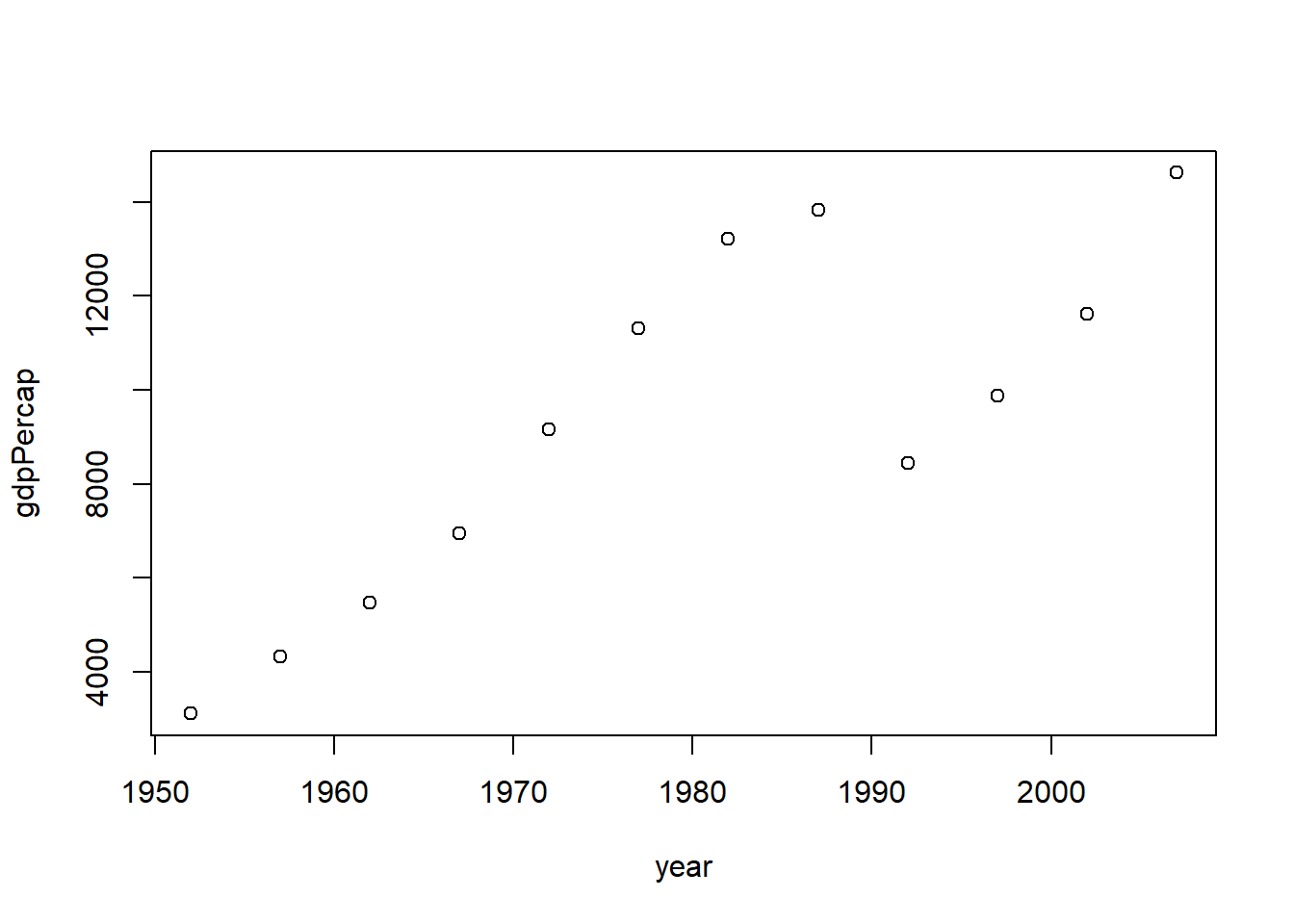
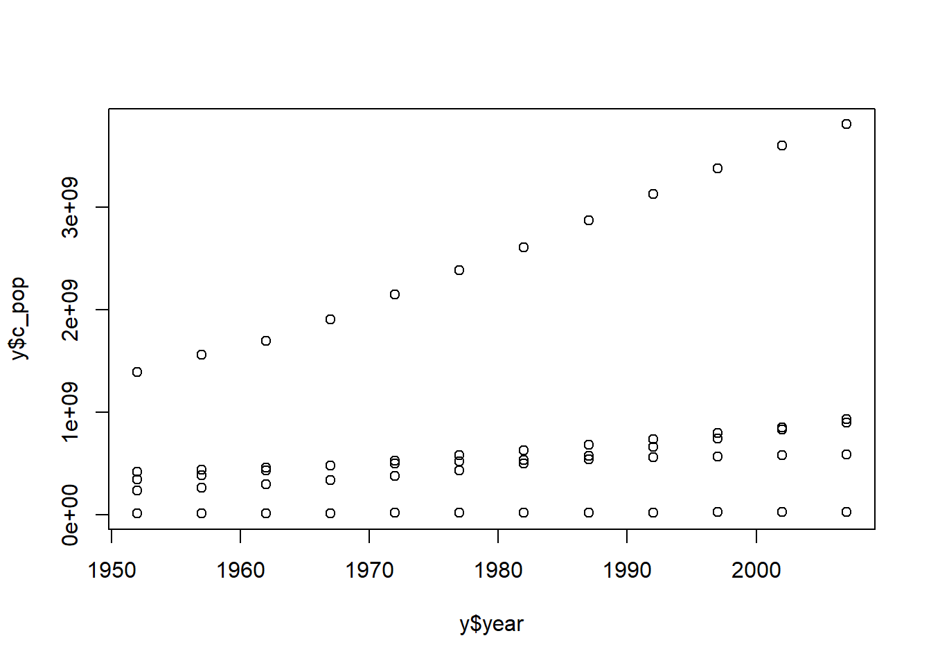
plot(y$year, y$c_pop)

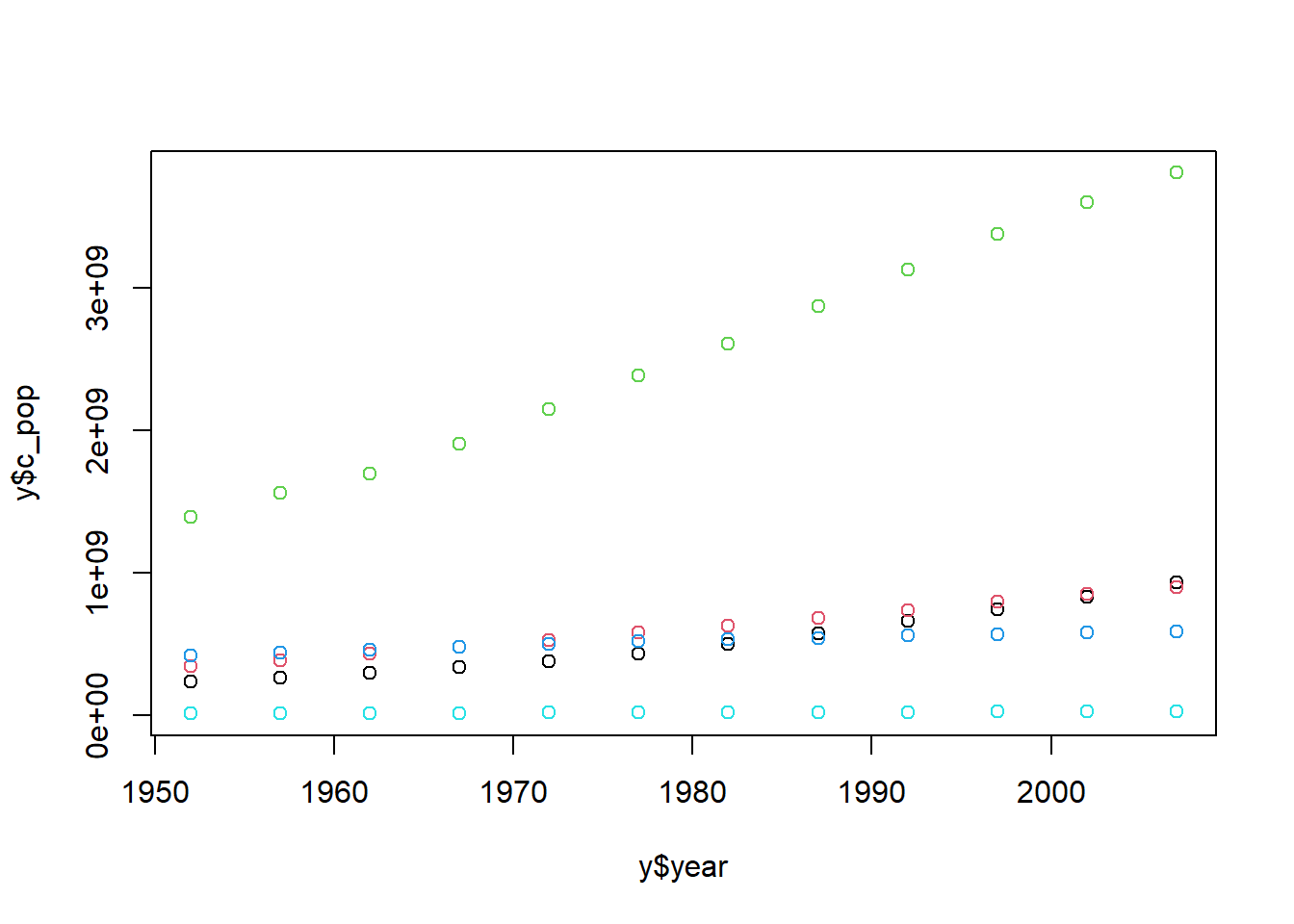
plot(y$year, y$c_pop, col = y$continent)

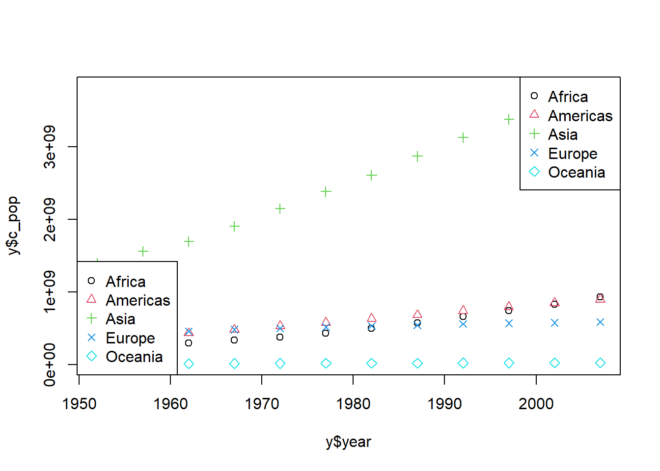
plot(y$year, y$c_pop, col = y$continent, pch = c(1:5))
plot(y$year, y$c_pop, col = y$continent, pch = c(1:length(levels(y$continent))))

# 범례 개수를 숫자로 지정
legend("topright", legend = levels((y$continent)), pch = c(1:5), col = c(1:5))

# 범례 개수를 데이터 개수에 맞게 지정
legend("bottomleft", legend = levels((y$continent)), pch = c(1:length(levels(y$continent))), col = c(1:length(levels(y$continent))))

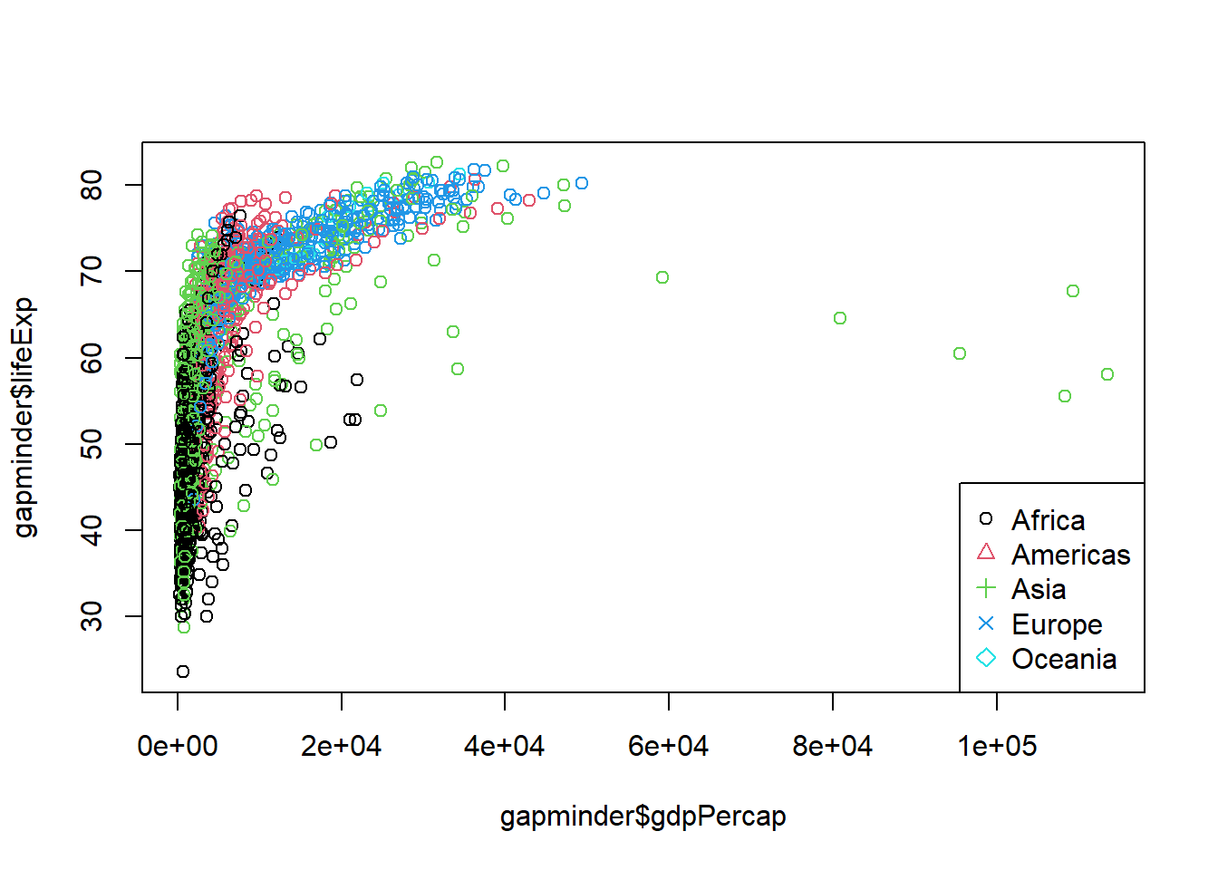
# 02 시각화의 기본 기능 #
plot(gapminder$gdpPercap, gapminder$lifeExp, col = gapminder$continent)
legend("bottomright", legend = levels((gapminder$continent)), 
       pch = c(1:length(levels(gapminder$continent))), 
       col = c(1:length(levels(y$continent))))

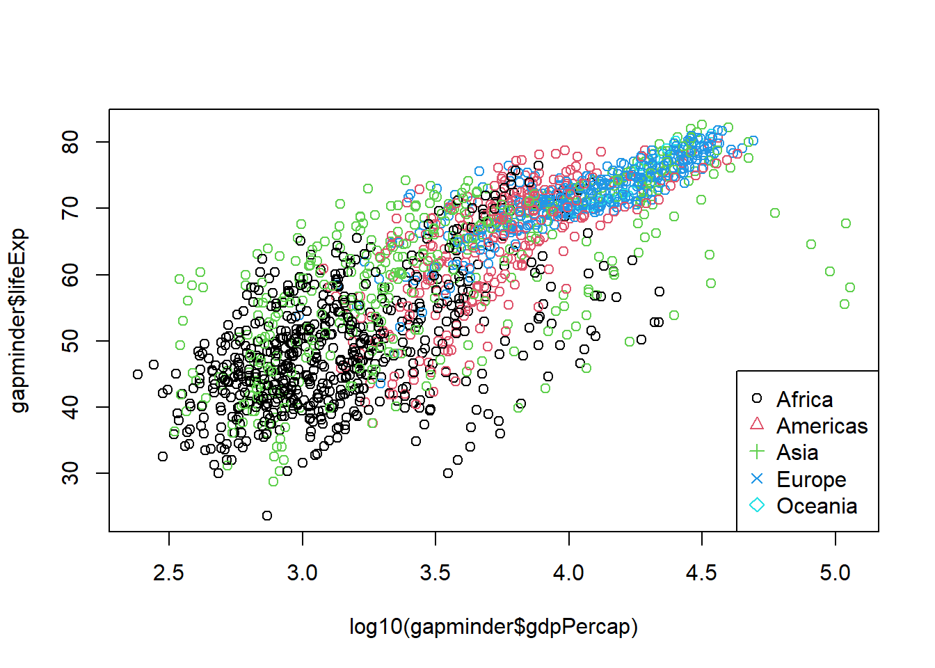
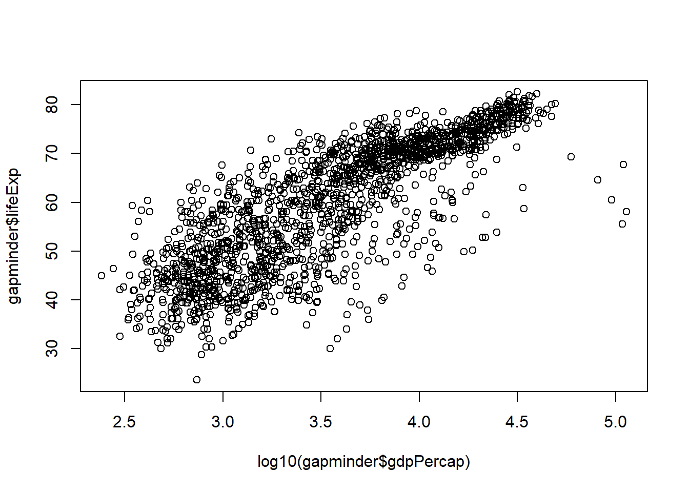
plot(log10(gapminder$gdpPercap), gapminder$lifeExp, col = gapminder$continent)
legend("bottomright", legend  = levels((gapminder$continent)), pch = c(1:length(levels(gapminder$continent))), col = c(1:length(levels(y$continent))))

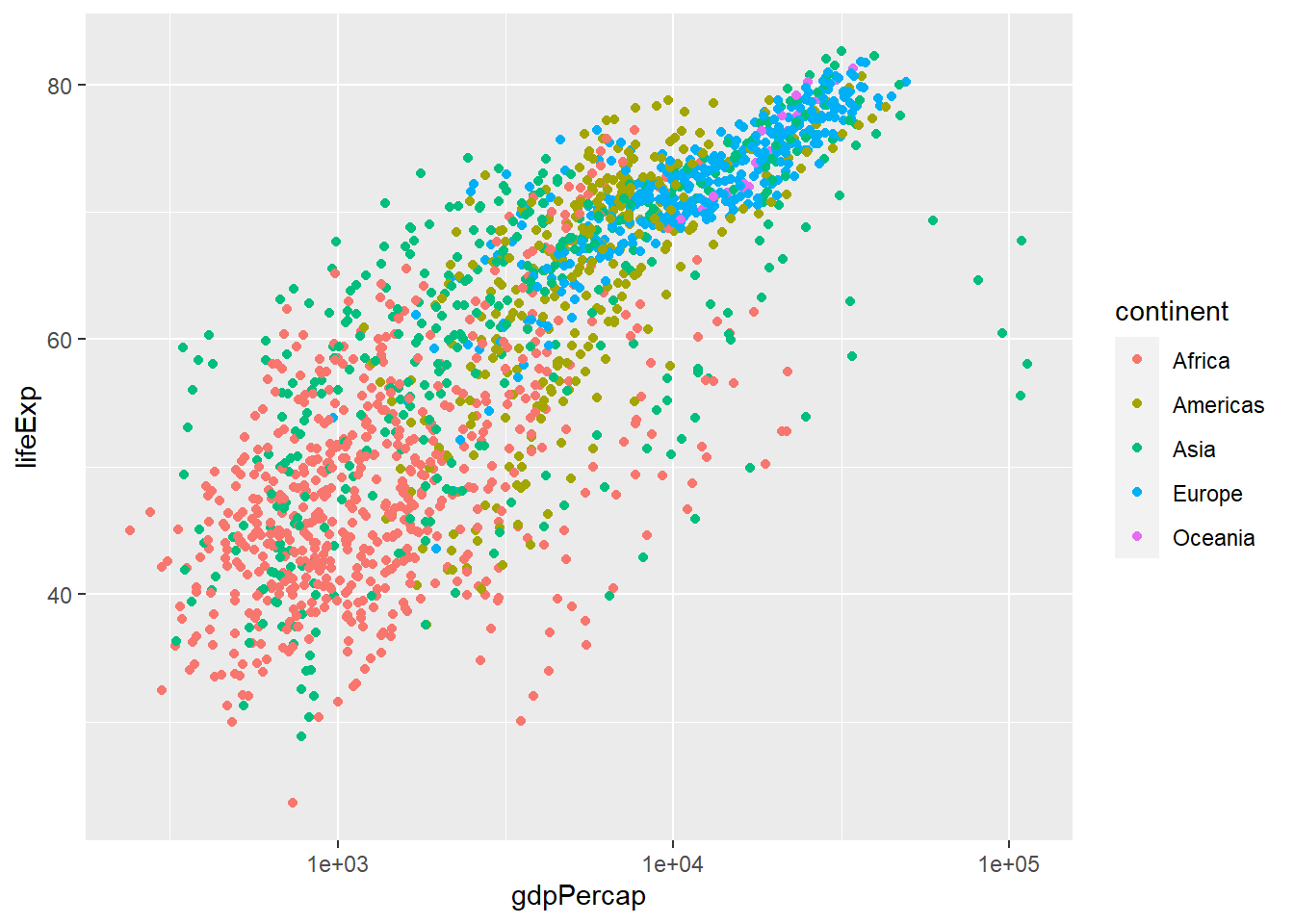
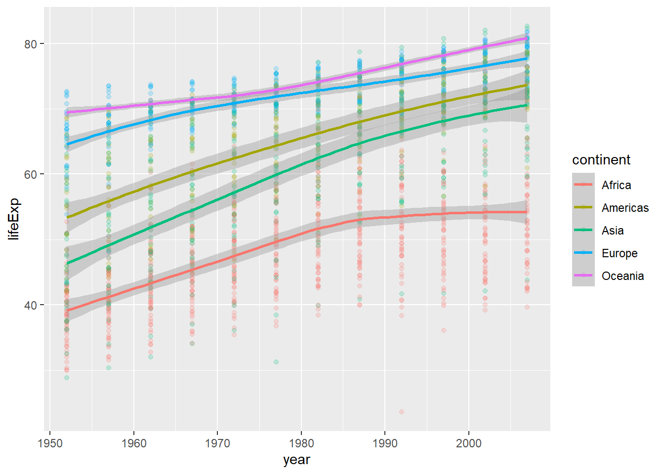
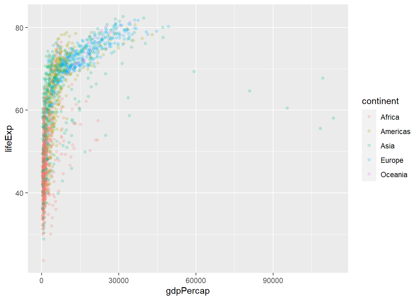
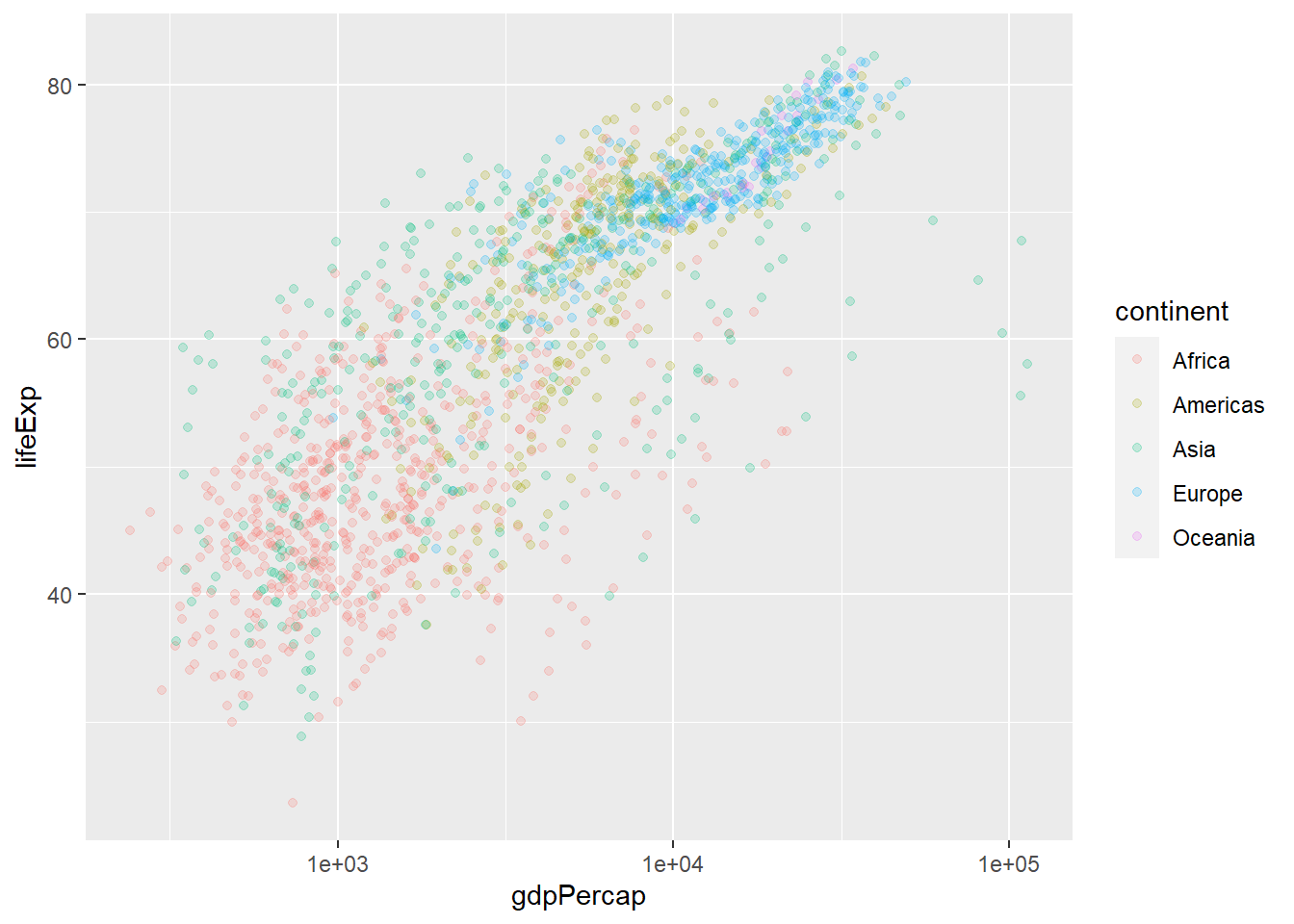
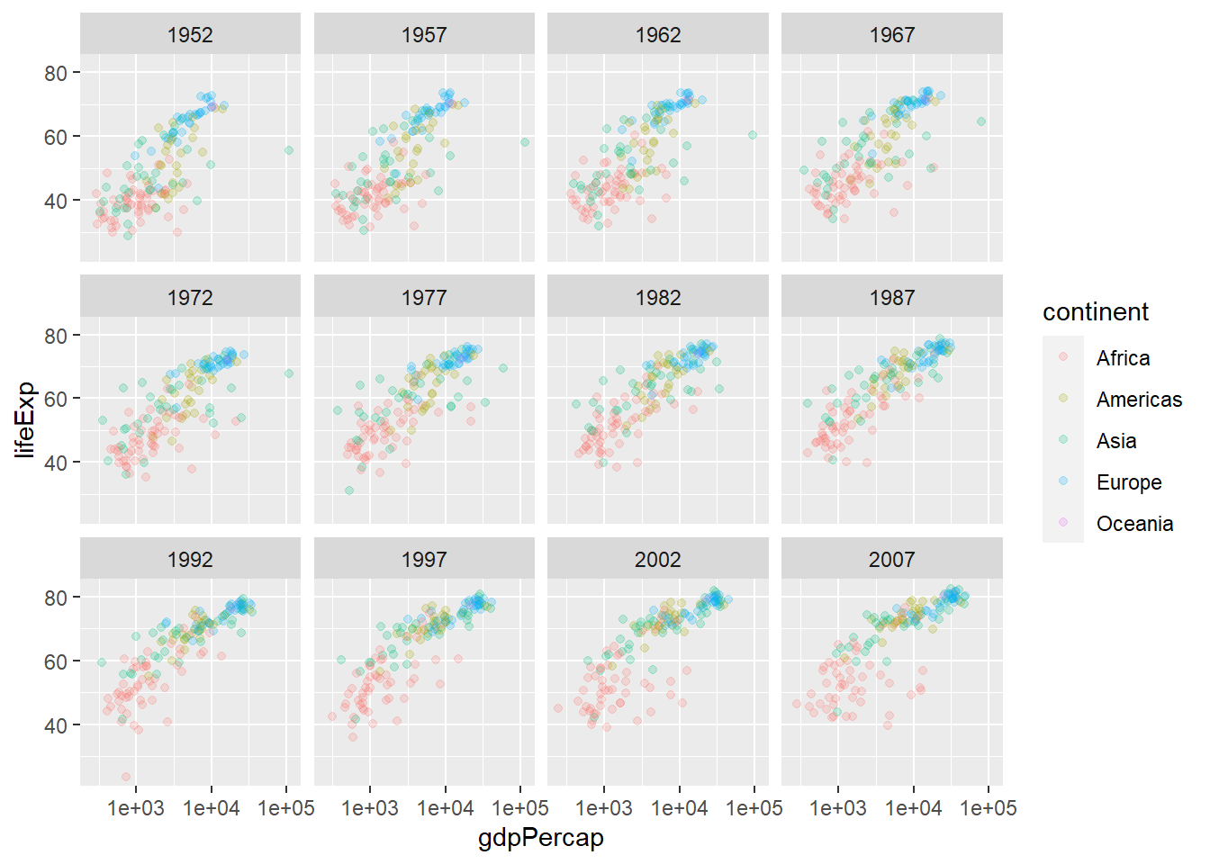
# install.packages("ggplot2")
library(ggplot2)
# gapminder %>% ggplot(,aes())

ggplot(gapminder, aes(x =  gdpPercap, y = lifeExp, col = continent)) + 
  geom_point() + 
  scale_x_log10()

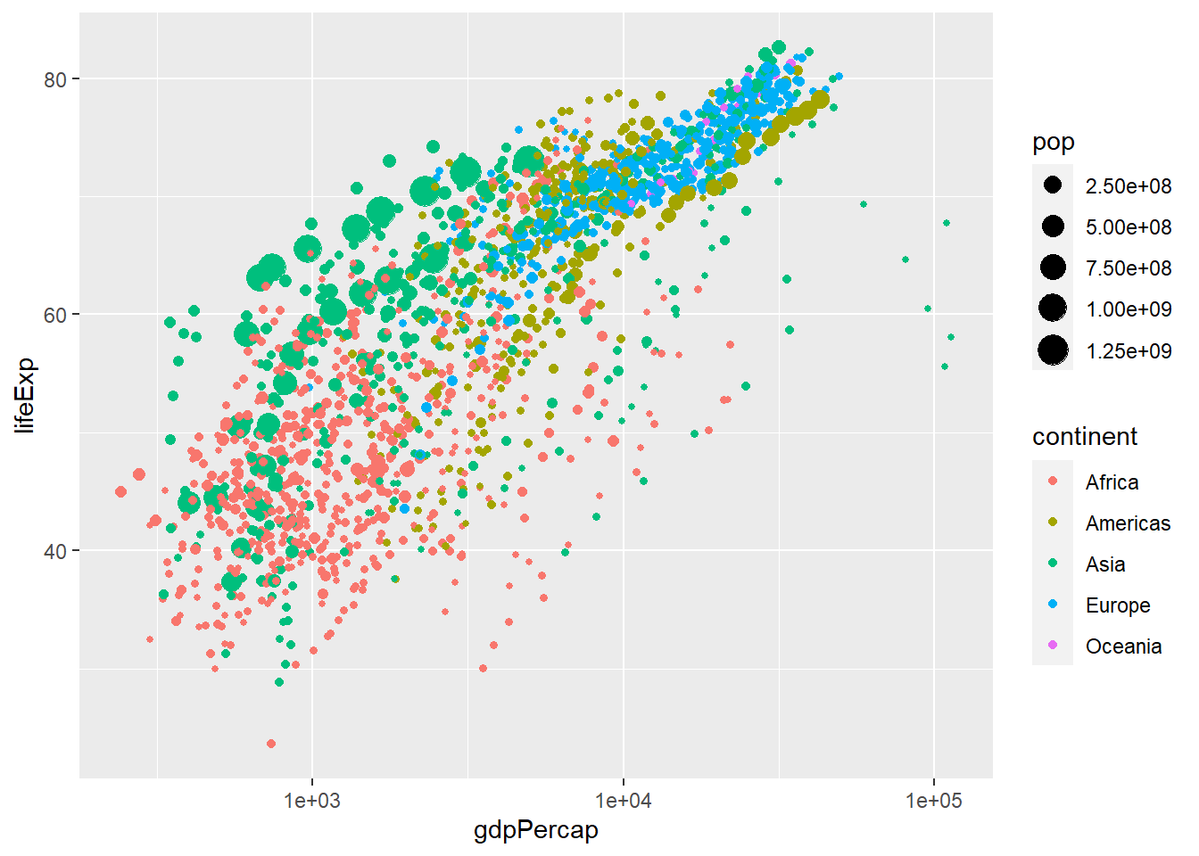
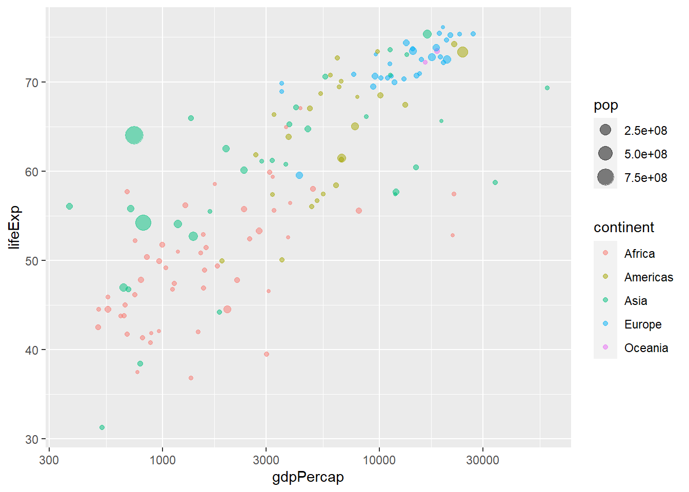
ggplot(gapminder, aes(x =  gdpPercap, y = lifeExp, col = continent, size = pop)) + 
  geom_point() + 
  scale_x_log10()

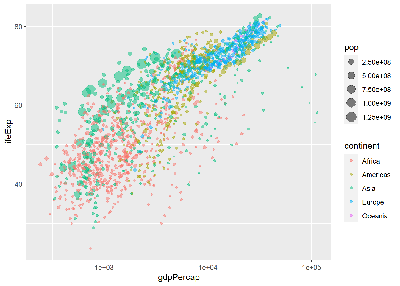
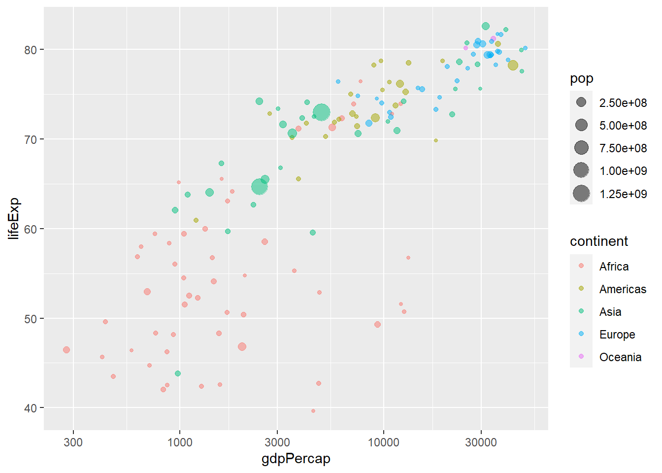
ggplot(gapminder, aes(x = gdpPercap, y = lifeExp, col = continent, size = pop)) + 
  geom_point(alpha = 0.5) + 
  scale_x_log10()

table(gapminder$year)

1952 1957 1962 1967 1972 1977 1982 1987 1992 1997 2002 2007 
 142  142  142  142  142  142  142  142  142  142  142  142 

gapminder %>% filter(year==1977) %>% 
  ggplot(., aes(x=gdpPercap, y=lifeExp, col=continent, size=pop)) + 
  geom_point(alpha=0.5) + 
  scale_x_log10() 

gapminder %>% filter(year==2007) %>% 
  ggplot(., aes(x=gdpPercap, y=lifeExp, col=continent, size=pop)) + 
  geom_point(alpha=0.5) + 
  scale_x_log10() 

ggplot(gapminder, aes(x=gdpPercap, y=lifeExp, col=continent, size=pop)) + 
  geom_point(alpha=0.5) + 
  scale_x_log10() + 
  facet_wrap(~year)

gapminder %>% 
  filter(year == 1952 & continent =="Asia") %>% 
  ggplot(aes(reorder(country, pop), pop)) + 
  geom_bar(stat = "identity") + 
  coord_flip()

gapminder %>% filter(year==1952 & continent== "Asia") %>% ggplot(aes(reorder(country, pop), pop)) + geom_bar(stat  = "identity") + scale_y_log10() + coord_flip()

gapminder %>% 
  filter(country == "Korea, Rep.") %>% 
  ggplot(aes(year, lifeExp, col = country)) + 
  geom_point() + 
  geom_line()

gapminder %>% 
  filter(country == "Korea, Rep.") %>% 
  ggplot(aes(year, lifeExp, col = country)) + 
  # geom_point() + 
  geom_line()

gapminder %>% 
  ggplot(aes(x = year, y = lifeExp, col = continent)) + 
  geom_point(alpha = 0.2) + 
  geom_smooth()

`geom_smooth()` using method = 'loess' and formula = 'y ~ x'

x = filter(gapminder, year == 1952)
hist(x$lifeExp, main = "Histogram of lifeExp in 1952")

x %>% ggplot(aes(lifeExp)) + geom_histogram()

`stat_bin()` using `bins = 30`. Pick better value with `binwidth`.

x %>% ggplot(aes(continent, lifeExp)) + geom_boxplot()

plot(log10(gapminder$gdpPercap), gapminder$lifeExp)

# 03 Visualization Tool

head(cars)

  speed dist
1     4    2
2     4   10
3     7    4
4     7   22
5     8   16
6     9   10

# type = "p"는 점 플롯, main = "cars"는 그래프의 제목
plot(cars, type  = "p", main  = "cars")

plot(cars, type = "l", main = "cars")       # type ="l"은 선을 사용한 플롯

plot(cars, type="b", main="cars")   # type ="b"는 점과 선을 모두 사용한 플롯

plot(cars, type = "h", main = "cars")  # type ="h"는 히스토그램과 같은 막대 그래프

x = gapminder %>% filter(year == 1952 & continent == "Asia") %>% mutate(gdp = gdpPercap*pop) %>% select(country, gdp) %>% arrange(desc(gdp)) %>% head()
pie(x$gdp, x$country)

barplot(x$gdp, names.arg = x$country)

x = gapminder %>% filter(year == 2007 & continent == "Asia") %>% mutate(gdp  = gdpPercap*pop) %>% select(country, gdp) %>% arrange(desc(gdp)) %>% head()
pie(x$gdp, x$country)

barplot(x$gdp, names.arg = x$country)

matplot(iris[, 1:4], type = "l")
legend("topleft", names(iris)[1:4], lty = c(1, 2, 3, 4), col = c(1, 2, 3, 4))

hist(cars$speed)

ggplot(gapminder, aes(x = gdpPercap, y = lifeExp, col = continent)) + geom_point(alpha = 0.2)

gapminder %>% filter(lifeExp>70) %>% 
  group_by(continent) %>% 
  summarize(n = n_distinct(country)) %>% 
  ggplot(aes(x = continent, y = n)) + 
  geom_bar(stat = "identity")

gapminder %>% filter(year == 2007) %>% 
  ggplot(aes(lifeExp, col = continent)) + 
  geom_histogram()

`stat_bin()` using `bins = 30`. Pick better value with `binwidth`.

gapminder %>% filter(year == 2007) %>% 
  ggplot(aes(lifeExp, col = continent)) + 
  geom_histogram(position = "dodge")

`stat_bin()` using `bins = 30`. Pick better value with `binwidth`.

gapminder %>% 
  filter(year == 2007) %>% 
  ggplot(aes(continent, lifeExp, col = continent)) + 
  geom_boxplot()

ggplot(gapminder, aes(x = gdpPercap, y = lifeExp, col = continent)) + 
  geom_point(alpha = 0.2)

ggplot(gapminder, aes(x = gdpPercap, y = lifeExp, col = continent)) +
  geom_point(alpha = 0.2) + scale_x_log10() # 가로축을 로그 스케일로 변환함.

gapminder %>% 
  filter(continent == "Africa") %>% 
  ggplot(aes(country, lifeExp)) + 
  geom_bar(stat  =  "identity")                  # [그림 6-35(a)]

gapminder %>% 
  filter(continent == "Africa") %>% 
  ggplot(aes(country, lifeExp)) + 
  geom_bar(stat  =  "identity") + 
  coord_flip()    # [그림 6-35(b)] 플롯의 방향을 전환함. 

# install.packages("RColorBrewer")
library(RColorBrewer)

display.brewer.all()

# [그림 6-37(a)] : 기본 팔레트를 적용한 그래프
gapminder %>% filter(lifeExp>70) %>% 
  group_by(continent) %>% 
  summarize(n  = n_distinct(country)) %>% 
  ggplot(aes(x = continent, y = n)) + 
  geom_bar(stat = "identity", aes(fill = continent)) 

# [그림 6-37(c)] Blues 팔레트를 적용한 그래프
gapminder %>% 
  filter(lifeExp>70) %>% 
  group_by(continent) %>% 
  summarize(n = n_distinct(country)) %>% 
  ggplot(aes(x = continent, y = n)) + 
  geom_bar(stat = "identity", aes(fill = continent)) + scale_fill_brewer(palette = "Blues")

# [그림 6-37(d)] Oranges 팔레트를 적용한 그래프
gapminder %>% 
  filter(lifeExp>70) %>% 
  group_by(continent) %>% 
  summarize(n =  n_distinct(country)) %>% 
  ggplot(aes(x = continent, y = n)) + 
  geom_bar(stat = "identity", aes(fill =  continent)) + scale_fill_brewer(palette = "Oranges")

# reorder(continent, -n)은 continent를 n을 기준으로 내림차 순으로 정렬하라는 의미
gapminder %>% 
  filter(lifeExp >70) %>% 
  group_by(continent) %>% 
  summarize(n  =  n_distinct(country)) %>% 
  ggplot(aes(x = reorder(continent, -n), y =  n)) + 
  geom_bar(stat = "identity", aes(fill =  continent)) + 
  scale_fill_brewer(palette  = "Blues")

# 실습!!
gapminder %>%
  filter(continent == "Africa", year==2007) %>%
  ggplot(aes(reorder(country, lifeExp), lifeExp, fill=lifeExp)) +
  geom_bar(stat  =  "identity") +
  coord_flip()

# 
gapminder %>%
  filter(continent == "Africa", year==2007) %>%
  ggplot(aes(reorder(country, lifeExp), lifeExp, fill=lifeExp)) +
  geom_bar(stat  =  "identity") +
  coord_flip()  + 
  scale_fill_distiller(palette = "Oranges", direction=1)

# 04 시각화를 이용한 데이터 탐색 #

gapminder %>% ggplot(aes(gdpPercap, lifeExp, col = continent)) + geom_point(alpha  =  0.2) + facet_wrap(~year) + scale_x_log10()

gapminder %>% filter(year == 1952 & gdpPercap > 10000 & continent == "Asia") 

# A tibble: 1 × 6
  country continent  year lifeExp    pop gdpPercap
  <fct>   <fct>     <int>   <dbl>  <int>     <dbl>
1 Kuwait  Asia       1952    55.6 160000   108382.

gapminder %>% filter(country == "Kuwait") %>% ggplot(aes(year, gdpPercap)) + geom_point() + geom_line()             # [그림 6-40(a)]

gapminder %>% filter(country == "Kuwait") %>% ggplot(aes(year, pop)) + geom_point() + geom_line()                   # [그림 6-40(b)]

gapminder %>% filter(country == "Korea, Rep.") %>% ggplot(aes(year, gdpPercap)) + geom_point() + geom_line()        # [그림 6-41(a)]

gapminder %>% filter(country == "Korea, Rep.") %>% ggplot(aes(year, pop)) + geom_point() + geom_line()              # [그림 6-41(b)]

gapminder %>% filter(country == "Kuwait" | country == "Korea, Rep.") %>% mutate(gdp = gdpPercap*pop) %>% ggplot(aes(year, gdp, col = country)) + geom_point() + geom_line()

# [그림 6-43(a)] gdpPercap의 변화 비교 
gapminder %>% filter(country == "Kuwait"|country == "Saudi Arabia"|country == "Iraq"|country == "Iran"|country == "Korea, Rep."|country == "China"|country == "Japan")  %>% ggplot(aes(year, gdpPercap, col = country)) + geom_point() + geom_line()

# [그림 6-43(b)] pop의 변화 비교 
gapminder %>% filter(country == "Kuwait"|country=="Saudi Arabia"|country == "Iraq"|country == "Iran"|country == "Korea, Rep."|country == "China"|country == "Japan")  %>% ggplot(aes(year, pop, col=country)) + geom_point() + geom_line()

# [그림 6-43(c)] gdp의 변화 비교 
gapminder %>% filter(country == "Kuwait"|country == "Saudi Arabia"|country == "Iraq"|country == "Iran"|country == "Korea, Rep."|country == "China"|country == "Japan")  %>% mutate(gdp=gdpPercap*pop) %>% ggplot(aes(year, gdp, col = country)) + geom_point() + geom_line() + scale_y_log10()