NLP

TF-IDF, 감정 분석

Comparing the frequency of words

Data import

library(tidyverse)

── Attaching core tidyverse packages ──────────────────────── tidyverse 2.0.0 ──
✔ dplyr     1.1.3     ✔ readr     2.1.4
✔ forcats   1.0.0     ✔ stringr   1.5.0
✔ ggplot2   3.4.4     ✔ tibble    3.2.1
✔ lubridate 1.9.3     ✔ tidyr     1.3.0
✔ purrr     1.0.2     
── Conflicts ────────────────────────────────────────── tidyverse_conflicts() ──
✖ dplyr::filter() masks stats::filter()
✖ dplyr::lag()    masks stats::lag()
ℹ Use the conflicted package (<http://conflicted.r-lib.org/>) to force all conflicts to become errors

raw_moon <- readLines('data/speech_moon.txt', encoding = 'UTF-8') # 문재인 대통령 연설문 불러오기
moon <- raw_moon %>% 
  as_tibble() %>% 
  mutate(president = 'moon')

raw_park <- readLines('data/speech_park.txt', encoding = 'UTF-8')
park <- raw_park %>% 
  as_tibble() %>% 
  mutate(president = 'park')

Data merge

# 데이터 합치기
bind_speeches <- bind_rows(moon, park) %>% 
  select(president, value)

head(bind_speeches)

# A tibble: 6 × 2
  president value                                                               
  <chr>     <chr>                                                               
1 moon      "정권교체 하겠습니다!"                                              
2 moon      "  정치교체 하겠습니다!"                                            
3 moon      "  시대교체 하겠습니다!"                                            
4 moon      "  "                                                                
5 moon      "  ‘불비불명(不飛不鳴)’이라는 고사가 있습니다. 남쪽 언덕 나뭇가지에…
6 moon      ""                                                                  

tail(bind_speeches)

# A tibble: 6 × 2
  president value                                                              
  <chr>     <chr>                                                              
1 park      "국민들이 꿈으로만 가졌던 행복한 삶을 실제로 이룰 수 있도록 도와드…
2 park      ""                                                                 
3 park      "감사합니다."                                                      
4 park      ""                                                                 
5 park      "2012년 7월 10일"                                                  
6 park      "새누리당 예비후보 박근혜"                                         

집단별 단어 빈도 구하기 1. 기본적인 전처리 및 토큰화

# 기본적인 전처리
library(stringr)
speeches <- bind_speeches %>% 
  mutate(value = str_replace_all(value, '[^가-힣]', ' '),
         value = str_squish(value))
speeches

# A tibble: 213 × 2
   president value                                                              
   <chr>     <chr>                                                              
 1 moon      "정권교체 하겠습니다"                                              
 2 moon      "정치교체 하겠습니다"                                              
 3 moon      "시대교체 하겠습니다"                                              
 4 moon      ""                                                                 
 5 moon      "불비불명 이라는 고사가 있습니다 남쪽 언덕 나뭇가지에 앉아 년 동안…
 6 moon      ""                                                                 
 7 moon      "그 동안 정치와 거리를 둬 왔습니다 그러나 암울한 시대가 저를 정치… 
 8 moon      ""                                                                 
 9 moon      ""                                                                 
10 moon      "우리나라 대통령 이 되겠습니다"                                    
# ℹ 203 more rows

Tokenization

# 토큰화
library(tidytext)
library(KoNLP)

Checking user defined dictionary!

speeches <- speeches %>% 
  unnest_tokens(input = value,
                output = word,
                token = extractNoun)
speeches

# A tibble: 2,997 × 2
   president word      
   <chr>     <chr>     
 1 moon      "정권교체"
 2 moon      "하겠습니"
 3 moon      "정치"    
 4 moon      "교체"    
 5 moon      "하겠습니"
 6 moon      "시대"    
 7 moon      "교체"    
 8 moon      "하겠습니"
 9 moon      ""        
10 moon      "불비불명"
# ℹ 2,987 more rows

하위 집단별 단어 빈도 구하기 - count()

# 샘플 텍스트로 작동 원리 알아보기
df <- tibble(class = c('a','a','a','b','b','b'),
             sex = c('female','male','female','male','male','female'))
df

# A tibble: 6 × 2
  class sex   
  <chr> <chr> 
1 a     female
2 a     male  
3 a     female
4 b     male  
5 b     male  
6 b     female

df %>% count(class, sex)

# A tibble: 4 × 3
  class sex        n
  <chr> <chr>  <int>
1 a     female     2
2 a     male       1
3 b     female     1
4 b     male       2

두 연설문의 단어 빈도 구하기

# 두 연설문의 단어 빈도 구하기
frequency <- speeches %>% 
  count(president, word) %>% 
  filter(str_count(word) > 1)
head(frequency)

# A tibble: 6 × 3
  president word         n
  <chr>     <chr>    <int>
1 moon      가동         1
2 moon      가사         1
3 moon      가슴         2
4 moon      가족         1
5 moon      가족구조     1
6 moon      가지         4

자주 사용된 단어 추출하기, dplyr::slice_max()

• 값이 큰 상위 n개의 행을 추출해 내림차순 정렬

# 샘플 텍스트로 작동 원리 알아보기
df <- tibble(x = c(1:100))
df

# A tibble: 100 × 1
       x
   <int>
 1     1
 2     2
 3     3
 4     4
 5     5
 6     6
 7     7
 8     8
 9     9
10    10
# ℹ 90 more rows

df %>% slice_max(x, n = 3)

# A tibble: 3 × 1
      x
  <int>
1   100
2    99
3    98

연설문에 가장 많이 사용된 단어 추출하기

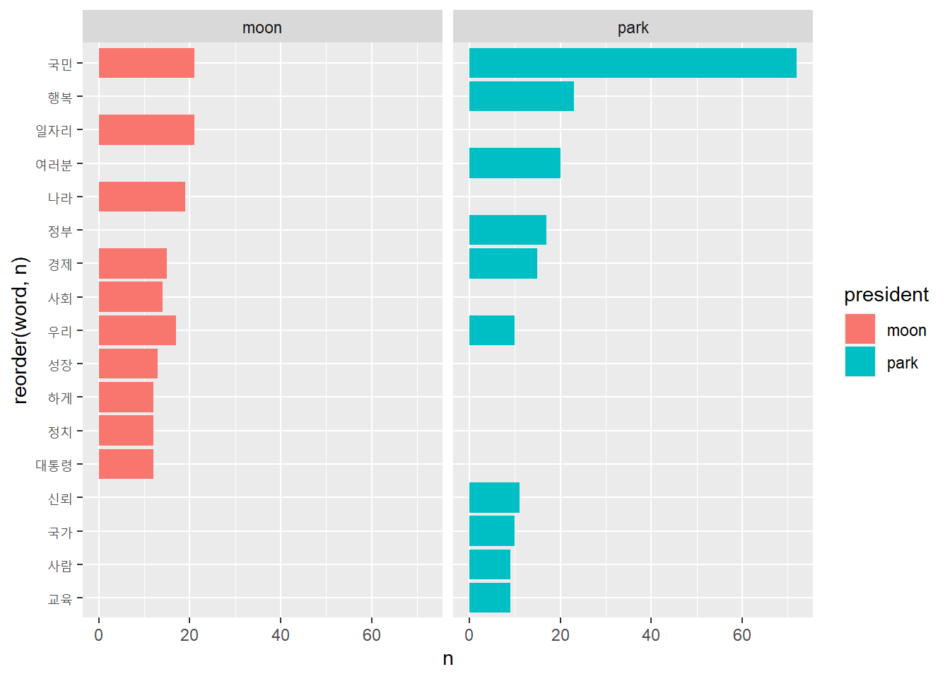
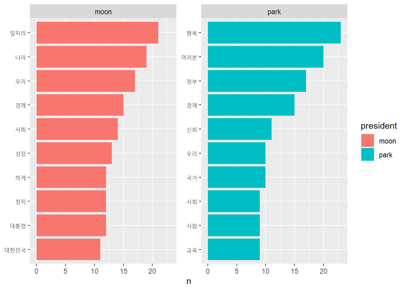
# 연설문에 가장 많이 사용된 단어 추출하기
top10 <- frequency %>% 
  group_by(president) %>% 
  slice_max(n, n = 10)
top10

# A tibble: 22 × 3
# Groups:   president [2]
   president word       n
   <chr>     <chr>  <int>
 1 moon      국민      21
 2 moon      일자리    21
 3 moon      나라      19
 4 moon      우리      17
 5 moon      경제      15
 6 moon      사회      14
 7 moon      성장      13
 8 moon      대통령    12
 9 moon      정치      12
10 moon      하게      12
# ℹ 12 more rows

# 단어 빈도 동점 처리 제외하고 추출하기, slice_max(with_ties = F) - 원본 데이터의 정렬 순서에 따라 행 추출
top10 %>% 
  filter(president == 'park') # 박근혜 전 대통령의 연설문은 동점 처리로 인해, 단어 12개가 모두 추출되어버림

# A tibble: 12 × 3
# Groups:   president [1]
   president word       n
   <chr>     <chr>  <int>
 1 park      국민      72
 2 park      행복      23
 3 park      여러분    20
 4 park      정부      17
 5 park      경제      15
 6 park      신뢰      11
 7 park      국가      10
 8 park      우리      10
 9 park      교육       9
10 park      사람       9
11 park      사회       9
12 park      일자리     9

# 샘플 데이터로 작동 원리 알아보기
df <- tibble(x = c('A','B','C','D'), y = c(4,3,2,2))
df %>% 
  slice_max(y, n = 3)

# A tibble: 4 × 2
  x         y
  <chr> <dbl>
1 A         4
2 B         3
3 C         2
4 D         2

df %>% 
  slice_max(y, n = 3, with_ties = F)

# A tibble: 3 × 2
  x         y
  <chr> <dbl>
1 A         4
2 B         3
3 C         2

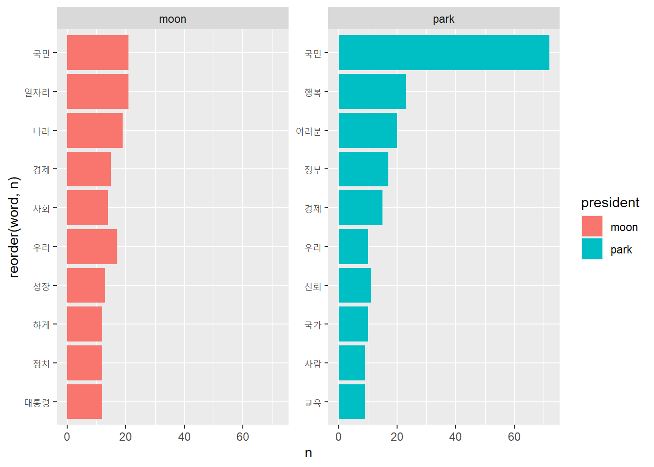
# 연설문에 적용하기
top10 <- frequency %>% 
  group_by(president) %>% 
  slice_max(n, n = 10, with_ties = F)
top10

# A tibble: 20 × 3
# Groups:   president [2]
   president word       n
   <chr>     <chr>  <int>
 1 moon      국민      21
 2 moon      일자리    21
 3 moon      나라      19
 4 moon      우리      17
 5 moon      경제      15
 6 moon      사회      14
 7 moon      성장      13
 8 moon      대통령    12
 9 moon      정치      12
10 moon      하게      12
11 park      국민      72
12 park      행복      23
13 park      여러분    20
14 park      정부      17
15 park      경제      15
16 park      신뢰      11
17 park      국가      10
18 park      우리      10
19 park      교육       9
20 park      사람       9

Visualization

# 막대 그래프 만들기
# 1. 변수의 항목별로 그래프 만들기 - facet_wrap()
ggplot(top10, aes(x = reorder(word, n),
                  y = n,
                  fill = president)) +
  geom_col() +
  coord_flip() +
  facet_wrap(~ president)

facet_wrap: scale free!

# 2. 그래프별 y축 설정하기
ggplot(top10, aes(x = reorder(word, n),
                  y = n,
                  fill = president)) +
  geom_col() +
  coord_flip() +
  facet_wrap(~ president, # president별 그래프 생성
             scales = 'free_y') # y축 통일하지 않음

# 3. 특정 단어 제외하고 막대 그래프 만들기
top10 <- frequency %>% 
  filter(word != '국민') %>% 
  group_by(president) %>% 
  slice_max(n, n = 10, with_ties = F)

ggplot(top10, aes(x = reorder(word, n),
                  y = n,
                  fill = president)) +
  geom_col() +
  coord_flip() +
  facet_wrap(~ president, scales = 'free_y')

reorder_within!

# 4. 축 정렬하기
ggplot(top10, aes(x = reorder_within(word, n, president),
                  y = n,
                  fill = president)) +
  geom_col() +
  coord_flip() +
  facet_wrap(~ president, scales = 'free_y')

# 5. 변수 항목 제거하기
ggplot(top10, aes(x = reorder_within(word, n, president),
                  y = n,
                  fill = president)) +
  geom_col() +
  coord_flip() +
  facet_wrap(~ president, scales = "free_y") +
  scale_x_reordered() +
  labs(x = NULL) 

Odds Ratio

상대적으로 중요한 단어 찾기

# Long form을 Wide form으로 변환하기
# Long form 데이터 살펴보기
df_long <- frequency %>% 
  group_by(president) %>% 
  slice_max(n, n = 10) %>% 
  filter(word %in% c('국민','우리','정치','행복'))
df_long

# A tibble: 6 × 3
# Groups:   president [2]
  president word      n
  <chr>     <chr> <int>
1 moon      국민     21
2 moon      우리     17
3 moon      정치     12
4 park      국민     72
5 park      행복     23
6 park      우리     10

# Long form을 Wide form으로 변형하기
df_wide <- df_long %>% 
  pivot_wider(names_from = president,
              values_from = n)
df_wide

# A tibble: 4 × 3
  word   moon  park
  <chr> <int> <int>
1 국민     21    72
2 우리     17    10
3 정치     12    NA
4 행복     NA    23

# NA를 0으로 바꾸기
df_wide <- df_long %>% 
  pivot_wider(names_from = president,
              values_from = n,
              values_fill = list(n = 0))
df_wide

# A tibble: 4 × 3
  word   moon  park
  <chr> <int> <int>
1 국민     21    72
2 우리     17    10
3 정치     12     0
4 행복      0    23

# 연설문 단어 빈도를 Wide form으로 변환하기
frequency_wide <- frequency %>% 
  pivot_wider(names_from = president,
              values_from = n,
              values_fill = list(n = 0))
frequency_wide

# A tibble: 955 × 3
   word      moon  park
   <chr>    <int> <int>
 1 가동         1     0
 2 가사         1     0
 3 가슴         2     0
 4 가족         1     1
 5 가족구조     1     0
 6 가지         4     0
 7 가치         3     1
 8 각종         1     0
 9 감당         1     0
10 강력         3     0
# ℹ 945 more rows

Odds Ratio!

# 오즈비 구하기
# 1. 단어의 비중을 나타낸 변수 추가하기
frequency_wide <- frequency_wide %>%
  mutate(ratio_moon = ((moon)/(sum(moon))), # moon 에서 단어의 비중
         ratio_park = ((park)/(sum(park)))) # park 에서 단어의 비중
frequency_wide

# A tibble: 955 × 5
   word      moon  park ratio_moon ratio_park
   <chr>    <int> <int>      <dbl>      <dbl>
 1 가동         1     0   0.000749    0      
 2 가사         1     0   0.000749    0      
 3 가슴         2     0   0.00150     0      
 4 가족         1     1   0.000749    0.00117
 5 가족구조     1     0   0.000749    0      
 6 가지         4     0   0.00299     0      
 7 가치         3     1   0.00225     0.00117
 8 각종         1     0   0.000749    0      
 9 감당         1     0   0.000749    0      
10 강력         3     0   0.00225     0      
# ℹ 945 more rows

# 어떤 단어가 한 연설문에 전혀 사용되지 않으면 빈도/오즈비 0, 단어 비중 비교 불가, 
#빈도가 0보다 큰 값이 되도록 모든 값에 +1
frequency_wide <- frequency_wide %>%
  mutate(ratio_moon = ((moon + 1)/(sum(moon + 1))), # moon에서 단어의 비중
         ratio_park = ((park + 1)/(sum(park + 1)))) # park에서 단어의 비중
frequency_wide

# A tibble: 955 × 5
   word      moon  park ratio_moon ratio_park
   <chr>    <int> <int>      <dbl>      <dbl>
 1 가동         1     0   0.000873   0.000552
 2 가사         1     0   0.000873   0.000552
 3 가슴         2     0   0.00131    0.000552
 4 가족         1     1   0.000873   0.00110 
 5 가족구조     1     0   0.000873   0.000552
 6 가지         4     0   0.00218    0.000552
 7 가치         3     1   0.00175    0.00110 
 8 각종         1     0   0.000873   0.000552
 9 감당         1     0   0.000873   0.000552
10 강력         3     0   0.00175    0.000552
# ℹ 945 more rows

Create a new odds ratio variable

# 2. 오즈비 변수 추가하기
frequency_wide <- frequency_wide %>% 
  mutate(odds_ratio = ratio_moon / ratio_park)
frequency_wide

# A tibble: 955 × 6
   word      moon  park ratio_moon ratio_park odds_ratio
   <chr>    <int> <int>      <dbl>      <dbl>      <dbl>
 1 가동         1     0   0.000873   0.000552      1.58 
 2 가사         1     0   0.000873   0.000552      1.58 
 3 가슴         2     0   0.00131    0.000552      2.37 
 4 가족         1     1   0.000873   0.00110       0.791
 5 가족구조     1     0   0.000873   0.000552      1.58 
 6 가지         4     0   0.00218    0.000552      3.96 
 7 가치         3     1   0.00175    0.00110       1.58 
 8 각종         1     0   0.000873   0.000552      1.58 
 9 감당         1     0   0.000873   0.000552      1.58 
10 강력         3     0   0.00175    0.000552      3.17 
# ℹ 945 more rows

frequency_wide %>% 
  arrange(-odds_ratio) # moon에서 상대적인 비중이 클수록 1보다 큰 값

# A tibble: 955 × 6
   word      moon  park ratio_moon ratio_park odds_ratio
   <chr>    <int> <int>      <dbl>      <dbl>      <dbl>
 1 복지국가     8     0    0.00393   0.000552       7.12
 2 세상         6     0    0.00306   0.000552       5.54
 3 여성         6     0    0.00306   0.000552       5.54
 4 정의         6     0    0.00306   0.000552       5.54
 5 강자         5     0    0.00262   0.000552       4.75
 6 공평         5     0    0.00262   0.000552       4.75
 7 대통령의     5     0    0.00262   0.000552       4.75
 8 보통         5     0    0.00262   0.000552       4.75
 9 상생         5     0    0.00262   0.000552       4.75
10 지방         5     0    0.00262   0.000552       4.75
# ℹ 945 more rows

frequency_wide %>% 
  arrange(odds_ratio) # park에서 상대적인 비중이 클수록 1보다 작은 값

# A tibble: 955 × 6
   word      moon  park ratio_moon ratio_park odds_ratio
   <chr>    <int> <int>      <dbl>      <dbl>      <dbl>
 1 박근혜       0     8   0.000436    0.00496     0.0879
 2 여러분       2    20   0.00131     0.0116      0.113 
 3 행복         3    23   0.00175     0.0132      0.132 
 4 실천         0     5   0.000436    0.00331     0.132 
 5 정보         0     5   0.000436    0.00331     0.132 
 6 투명         0     5   0.000436    0.00331     0.132 
 7 과제         0     4   0.000436    0.00276     0.158 
 8 국정운영     0     4   0.000436    0.00276     0.158 
 9 시작         0     4   0.000436    0.00276     0.158 
10 지식         0     4   0.000436    0.00276     0.158 
# ℹ 945 more rows

frequency_wide %>% 
  arrange(abs(1-odds_ratio)) # 두 연설문에서 단어 비중이 같으면 1

# A tibble: 955 × 6
   word    moon  park ratio_moon ratio_park odds_ratio
   <chr>  <int> <int>      <dbl>      <dbl>      <dbl>
 1 때문       4     3    0.00218    0.00221      0.989
 2 강화       3     2    0.00175    0.00165      1.06 
 3 부담       3     2    0.00175    0.00165      1.06 
 4 세계       3     2    0.00175    0.00165      1.06 
 5 책임       3     2    0.00175    0.00165      1.06 
 6 협력       3     2    0.00175    0.00165      1.06 
 7 거대       2     1    0.00131    0.00110      1.19 
 8 교체       2     1    0.00131    0.00110      1.19 
 9 근본적     2     1    0.00131    0.00110      1.19 
10 기반       2     1    0.00131    0.00110      1.19 
# ℹ 945 more rows

# 상대적으로 중요한 단어 추출하기
# 오즈비가 가장 높거나 가장 낮은 단어 추출하기
top10 <- frequency_wide %>% 
  filter(rank(odds_ratio) <= 10 | rank(-odds_ratio) <= 10)

top10 %>% 
  arrange(-odds_ratio)

# A tibble: 20 × 6
   word      moon  park ratio_moon ratio_park odds_ratio
   <chr>    <int> <int>      <dbl>      <dbl>      <dbl>
 1 복지국가     8     0   0.00393    0.000552     7.12  
 2 세상         6     0   0.00306    0.000552     5.54  
 3 여성         6     0   0.00306    0.000552     5.54  
 4 정의         6     0   0.00306    0.000552     5.54  
 5 강자         5     0   0.00262    0.000552     4.75  
 6 공평         5     0   0.00262    0.000552     4.75  
 7 대통령의     5     0   0.00262    0.000552     4.75  
 8 보통         5     0   0.00262    0.000552     4.75  
 9 상생         5     0   0.00262    0.000552     4.75  
10 지방         5     0   0.00262    0.000552     4.75  
11 과제         0     4   0.000436   0.00276      0.158 
12 국정운영     0     4   0.000436   0.00276      0.158 
13 시작         0     4   0.000436   0.00276      0.158 
14 지식         0     4   0.000436   0.00276      0.158 
15 행복         3    23   0.00175    0.0132       0.132 
16 실천         0     5   0.000436   0.00331      0.132 
17 정보         0     5   0.000436   0.00331      0.132 
18 투명         0     5   0.000436   0.00331      0.132 
19 여러분       2    20   0.00131    0.0116       0.113 
20 박근혜       0     8   0.000436   0.00496      0.0879

Visualization of relative importance

# 막대 그래프 만들기
# 1. 비중이 큰 연설문을 나타낸 변수 추가하기
top10 <- top10 %>%
  mutate(president = ifelse(odds_ratio > 1, "moon", "park"),
         n = ifelse(odds_ratio > 1, moon, park))
top10

# A tibble: 20 × 8
   word      moon  park ratio_moon ratio_park odds_ratio president     n
   <chr>    <int> <int>      <dbl>      <dbl>      <dbl> <chr>     <int>
 1 강자         5     0   0.00262    0.000552     4.75   moon          5
 2 공평         5     0   0.00262    0.000552     4.75   moon          5
 3 대통령의     5     0   0.00262    0.000552     4.75   moon          5
 4 보통         5     0   0.00262    0.000552     4.75   moon          5
 5 복지국가     8     0   0.00393    0.000552     7.12   moon          8
 6 상생         5     0   0.00262    0.000552     4.75   moon          5
 7 세상         6     0   0.00306    0.000552     5.54   moon          6
 8 여러분       2    20   0.00131    0.0116       0.113  park         20
 9 여성         6     0   0.00306    0.000552     5.54   moon          6
10 정의         6     0   0.00306    0.000552     5.54   moon          6
11 지방         5     0   0.00262    0.000552     4.75   moon          5
12 행복         3    23   0.00175    0.0132       0.132  park         23
13 과제         0     4   0.000436   0.00276      0.158  park          4
14 국정운영     0     4   0.000436   0.00276      0.158  park          4
15 박근혜       0     8   0.000436   0.00496      0.0879 park          8
16 시작         0     4   0.000436   0.00276      0.158  park          4
17 실천         0     5   0.000436   0.00331      0.132  park          5
18 정보         0     5   0.000436   0.00331      0.132  park          5
19 지식         0     4   0.000436   0.00276      0.158  park          4
20 투명         0     5   0.000436   0.00331      0.132  park          5

# 2. 막대 그래프 만들기
ggplot(top10, aes(x = reorder_within(word, n, president),
                  y = n,
                  fill = president)) +
  geom_col() +
  coord_flip() +
  facet_wrap(~ president, scales = 'free_y') +
  scale_x_reordered()

# 3. 그래프별로 축 설정하기
ggplot(top10, aes(x = reorder_within(word, n, president),
                  y = n,
                  fill = president)) +
  geom_col() +
  coord_flip() +
  facet_wrap(~ president, scales = "free") +
  scale_x_reordered() +
  labs(x = NULL) 

주요 단어가 사용된 문장 살펴보기

# 1. 원문을 문장 기준으로 토큰화하기
speeches_sentence <- bind_speeches %>% 
  as_tibble() %>% 
  unnest_tokens(input = value,
                output = sentence,
                token = 'sentences')
speeches_sentence

# A tibble: 329 × 2
   president sentence                                                          
   <chr>     <chr>                                                             
 1 moon      "정권교체 하겠습니다!"                                            
 2 moon      "정치교체 하겠습니다!"                                            
 3 moon      "시대교체 하겠습니다!"                                            
 4 moon      ""                                                                
 5 moon      "‘불비불명(不飛不鳴)’이라는 고사가 있습니다."                     
 6 moon      "남쪽 언덕 나뭇가지에 앉아, 3년 동안 날지도 울지도 않는 새."      
 7 moon      "그러나 그 새는 한번 날면 하늘 끝까지 날고, 한번 울면 천지를 뒤흔…
 8 moon      "그 동안 정치와 거리를 둬 왔습니다."                              
 9 moon      "그러나 암울한 시대가 저를 정치로 불러냈습니다."                  
10 moon      "더 이상 남쪽 나뭇가지에 머무를 수 없었습니다."                   
# ℹ 319 more rows

head(speeches_sentence)

# A tibble: 6 × 2
  president sentence                                                    
  <chr>     <chr>                                                       
1 moon      "정권교체 하겠습니다!"                                      
2 moon      "정치교체 하겠습니다!"                                      
3 moon      "시대교체 하겠습니다!"                                      
4 moon      ""                                                          
5 moon      "‘불비불명(不飛不鳴)’이라는 고사가 있습니다."               
6 moon      "남쪽 언덕 나뭇가지에 앉아, 3년 동안 날지도 울지도 않는 새."

tail(speeches_sentence)

# A tibble: 6 × 2
  president sentence                                                           
  <chr>     <chr>                                                              
1 park      국민 여러분의 행복이 곧 저의 행복입니다.                           
2 park      사랑하는 조국 대한민국과 국민 여러분을 위해, 앞으로 머나 먼 길, 끝…
3 park      그 길을 함께 해주시길 부탁드립니다.                                
4 park      감사합니다.                                                        
5 park      2012년 7월 10일                                                    
6 park      새누리당 예비후보 박근혜                                           

# 2. 주요 단어가 사용된 문장 추출하기 - str_detect()
speeches_sentence %>% 
  filter(president == 'moon' & str_detect(sentence, '복지국가'))

# A tibble: 8 × 2
  president sentence                                                            
  <chr>     <chr>                                                               
1 moon      ‘강한 복지국가’를 향해 담대하게 나아가겠습니다.                     
2 moon      2백 년 전 이와 같은 소득재분배, 복지국가의 사상을 가진 위정자가 지… 
3 moon      이제 우리는 복지국가를 향해 담대하게 나아갈 때입니다.               
4 moon      부자감세, 4대강 사업 같은 시대착오적 과오를 청산하고, 하루빨리 복지…
5 moon      우리는 지금 복지국가로 가느냐, 양극화의 분열된 국가로 가느냐 하는 … 
6 moon      강한 복지국가일수록 국가 경쟁력도 더 높습니다.                      
7 moon      결국 복지국가로 가는 길은 사람에 대한 투자, 일자리 창출, 자영업 고… 
8 moon      우리는 과감히 강한 보편적 복지국가로 가야 합니다.                   

두 연설문 모두에서 중요했던 단어들은?

# 중요도가 비슷한 단어 살펴보기
frequency_wide %>% 
  arrange(abs(1 - odds_ratio)) %>% 
  head(10)

# A tibble: 10 × 6
   word    moon  park ratio_moon ratio_park odds_ratio
   <chr>  <int> <int>      <dbl>      <dbl>      <dbl>
 1 때문       4     3    0.00218    0.00221      0.989
 2 강화       3     2    0.00175    0.00165      1.06 
 3 부담       3     2    0.00175    0.00165      1.06 
 4 세계       3     2    0.00175    0.00165      1.06 
 5 책임       3     2    0.00175    0.00165      1.06 
 6 협력       3     2    0.00175    0.00165      1.06 
 7 거대       2     1    0.00131    0.00110      1.19 
 8 교체       2     1    0.00131    0.00110      1.19 
 9 근본적     2     1    0.00131    0.00110      1.19 
10 기반       2     1    0.00131    0.00110      1.19 

# 중요도가 비슷하면서 빈도가 높은 단어
frequency_wide %>% 
  filter(moon >= 5 & park >= 5) %>%
  arrange(abs(1 - odds_ratio)) %>%
  head(10)

# A tibble: 10 × 6
   word      moon  park ratio_moon ratio_park odds_ratio
   <chr>    <int> <int>      <dbl>      <dbl>      <dbl>
 1 사회        14     9    0.00655    0.00552      1.19 
 2 사람         9     9    0.00436    0.00552      0.791
 3 경제        15    15    0.00698    0.00883      0.791
 4 지원         5     5    0.00262    0.00331      0.791
 5 우리        17    10    0.00786    0.00607      1.29 
 6 불안         7     8    0.00349    0.00496      0.703
 7 산업         9     5    0.00436    0.00331      1.32 
 8 대한민국    11     6    0.00524    0.00386      1.36 
 9 국가         7    10    0.00349    0.00607      0.576
10 교육         6     9    0.00306    0.00552      0.554

Log Odds Ratio

# 로그 오즈비 구하기
frequency_wide <- frequency_wide %>% 
  mutate(log_odds_ratio = log(odds_ratio))
frequency_wide

# A tibble: 955 × 7
   word      moon  park ratio_moon ratio_park odds_ratio log_odds_ratio
   <chr>    <int> <int>      <dbl>      <dbl>      <dbl>          <dbl>
 1 가동         1     0   0.000873   0.000552      1.58           0.459
 2 가사         1     0   0.000873   0.000552      1.58           0.459
 3 가슴         2     0   0.00131    0.000552      2.37           0.865
 4 가족         1     1   0.000873   0.00110       0.791         -0.234
 5 가족구조     1     0   0.000873   0.000552      1.58           0.459
 6 가지         4     0   0.00218    0.000552      3.96           1.38 
 7 가치         3     1   0.00175    0.00110       1.58           0.459
 8 각종         1     0   0.000873   0.000552      1.58           0.459
 9 감당         1     0   0.000873   0.000552      1.58           0.459
10 강력         3     0   0.00175    0.000552      3.17           1.15 
# ℹ 945 more rows

# moon에서 비중이 큰 단어, 0보다 큰 양수
frequency_wide %>%
  arrange(-log_odds_ratio)

# A tibble: 955 × 7
   word      moon  park ratio_moon ratio_park odds_ratio log_odds_ratio
   <chr>    <int> <int>      <dbl>      <dbl>      <dbl>          <dbl>
 1 복지국가     8     0    0.00393   0.000552       7.12           1.96
 2 세상         6     0    0.00306   0.000552       5.54           1.71
 3 여성         6     0    0.00306   0.000552       5.54           1.71
 4 정의         6     0    0.00306   0.000552       5.54           1.71
 5 강자         5     0    0.00262   0.000552       4.75           1.56
 6 공평         5     0    0.00262   0.000552       4.75           1.56
 7 대통령의     5     0    0.00262   0.000552       4.75           1.56
 8 보통         5     0    0.00262   0.000552       4.75           1.56
 9 상생         5     0    0.00262   0.000552       4.75           1.56
10 지방         5     0    0.00262   0.000552       4.75           1.56
# ℹ 945 more rows

# park에서 비중이 큰 단어, 0보다 작은 음수
frequency_wide %>%
  arrange(log_odds_ratio)

# A tibble: 955 × 7
   word      moon  park ratio_moon ratio_park odds_ratio log_odds_ratio
   <chr>    <int> <int>      <dbl>      <dbl>      <dbl>          <dbl>
 1 박근혜       0     8   0.000436    0.00496     0.0879          -2.43
 2 여러분       2    20   0.00131     0.0116      0.113           -2.18
 3 행복         3    23   0.00175     0.0132      0.132           -2.03
 4 실천         0     5   0.000436    0.00331     0.132           -2.03
 5 정보         0     5   0.000436    0.00331     0.132           -2.03
 6 투명         0     5   0.000436    0.00331     0.132           -2.03
 7 과제         0     4   0.000436    0.00276     0.158           -1.84
 8 국정운영     0     4   0.000436    0.00276     0.158           -1.84
 9 시작         0     4   0.000436    0.00276     0.158           -1.84
10 지식         0     4   0.000436    0.00276     0.158           -1.84
# ℹ 945 more rows

# 비중이 비슷한 단어, 0에 가까운
frequency_wide %>%
  arrange(abs(log_odds_ratio))

# A tibble: 955 × 7
   word    moon  park ratio_moon ratio_park odds_ratio log_odds_ratio
   <chr>  <int> <int>      <dbl>      <dbl>      <dbl>          <dbl>
 1 때문       4     3    0.00218    0.00221      0.989        -0.0109
 2 강화       3     2    0.00175    0.00165      1.06          0.0537
 3 부담       3     2    0.00175    0.00165      1.06          0.0537
 4 세계       3     2    0.00175    0.00165      1.06          0.0537
 5 책임       3     2    0.00175    0.00165      1.06          0.0537
 6 협력       3     2    0.00175    0.00165      1.06          0.0537
 7 거대       2     1    0.00131    0.00110      1.19          0.171 
 8 교체       2     1    0.00131    0.00110      1.19          0.171 
 9 근본적     2     1    0.00131    0.00110      1.19          0.171 
10 기반       2     1    0.00131    0.00110      1.19          0.171 
# ℹ 945 more rows

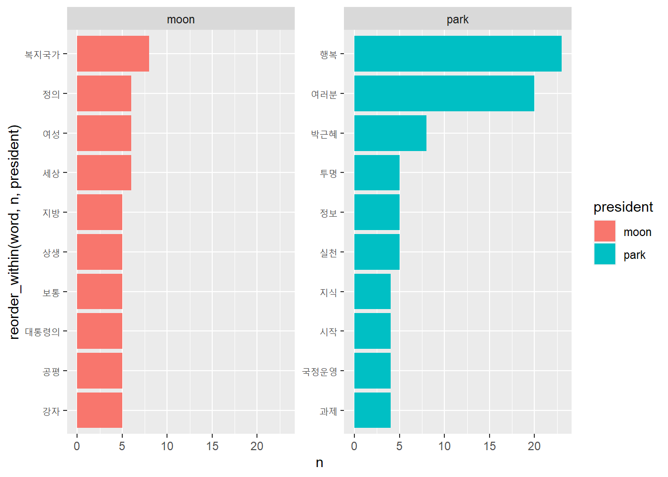
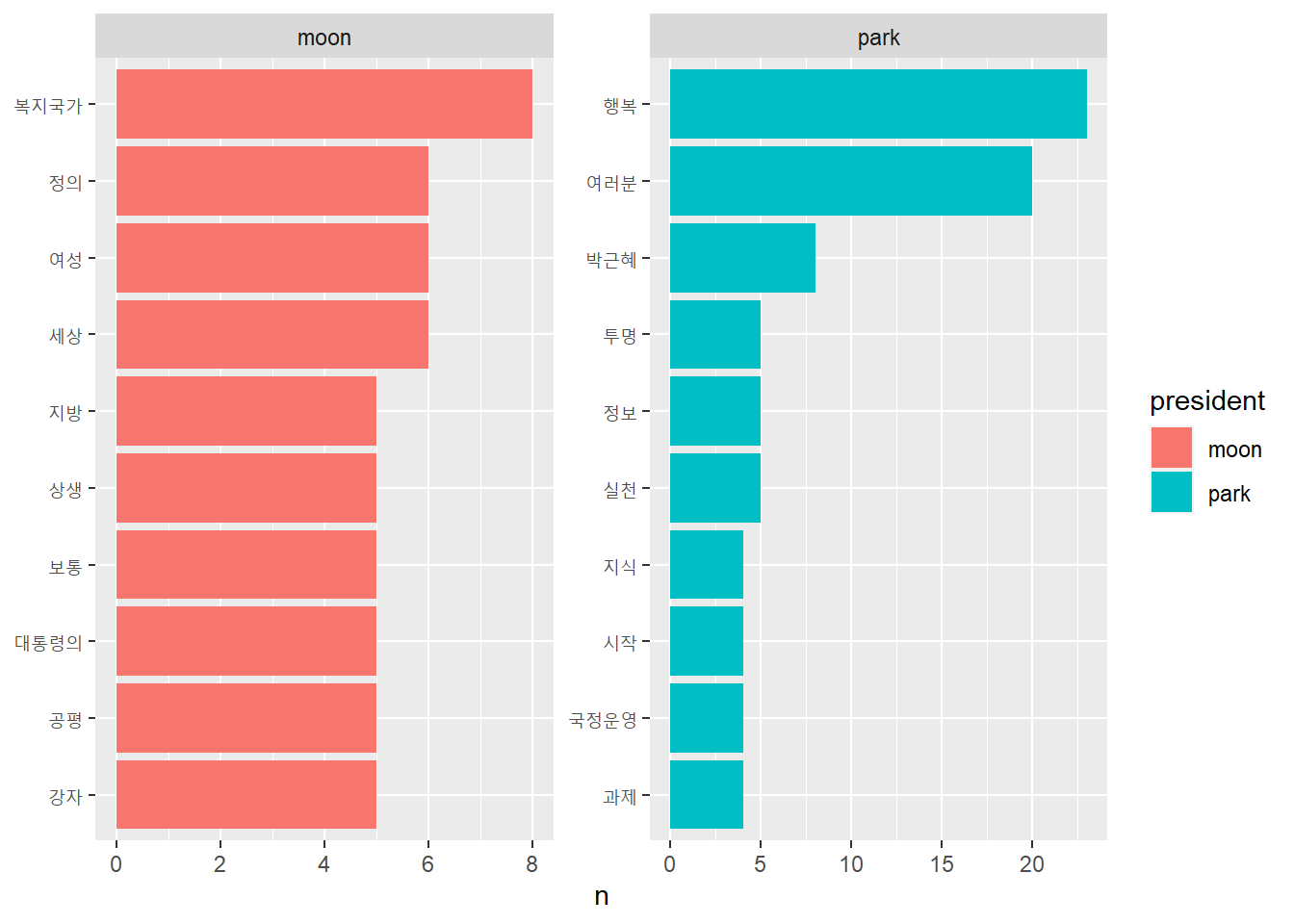
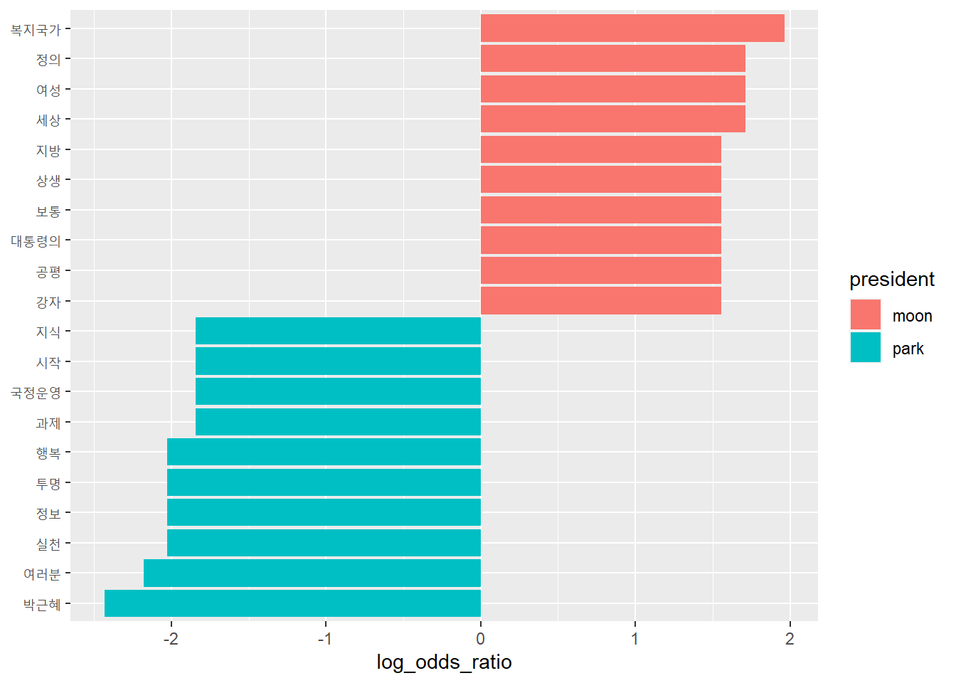
# 로그 오즈비를 이용해 중요한 단어 비교하기
top10 <- frequency_wide %>% 
  group_by(president = ifelse(log_odds_ratio > 0, 'moon', 'park')) %>% 
  slice_max(abs(log_odds_ratio), n = 10, with_ties = F)
top10

# A tibble: 20 × 8
# Groups:   president [2]
   word     moon  park ratio_moon ratio_park odds_ratio log_odds_ratio president
   <chr>   <int> <int>      <dbl>      <dbl>      <dbl>          <dbl> <chr>    
 1 복지국…     8     0   0.00393    0.000552     7.12             1.96 moon     
 2 세상        6     0   0.00306    0.000552     5.54             1.71 moon     
 3 여성        6     0   0.00306    0.000552     5.54             1.71 moon     
 4 정의        6     0   0.00306    0.000552     5.54             1.71 moon     
 5 강자        5     0   0.00262    0.000552     4.75             1.56 moon     
 6 공평        5     0   0.00262    0.000552     4.75             1.56 moon     
 7 대통령…     5     0   0.00262    0.000552     4.75             1.56 moon     
 8 보통        5     0   0.00262    0.000552     4.75             1.56 moon     
 9 상생        5     0   0.00262    0.000552     4.75             1.56 moon     
10 지방        5     0   0.00262    0.000552     4.75             1.56 moon     
11 박근혜      0     8   0.000436   0.00496      0.0879          -2.43 park     
12 여러분      2    20   0.00131    0.0116       0.113           -2.18 park     
13 행복        3    23   0.00175    0.0132       0.132           -2.03 park     
14 실천        0     5   0.000436   0.00331      0.132           -2.03 park     
15 정보        0     5   0.000436   0.00331      0.132           -2.03 park     
16 투명        0     5   0.000436   0.00331      0.132           -2.03 park     
17 과제        0     4   0.000436   0.00276      0.158           -1.84 park     
18 국정운…     0     4   0.000436   0.00276      0.158           -1.84 park     
19 시작        0     4   0.000436   0.00276      0.158           -1.84 park     
20 지식        0     4   0.000436   0.00276      0.158           -1.84 park     

# 주요 변수 추출
top10 %>%
  arrange(-log_odds_ratio) %>%
  select(word, log_odds_ratio, president)

# A tibble: 20 × 3
# Groups:   president [2]
   word     log_odds_ratio president
   <chr>             <dbl> <chr>    
 1 복지국가           1.96 moon     
 2 세상               1.71 moon     
 3 여성               1.71 moon     
 4 정의               1.71 moon     
 5 강자               1.56 moon     
 6 공평               1.56 moon     
 7 대통령의           1.56 moon     
 8 보통               1.56 moon     
 9 상생               1.56 moon     
10 지방               1.56 moon     
11 과제              -1.84 park     
12 국정운영          -1.84 park     
13 시작              -1.84 park     
14 지식              -1.84 park     
15 행복              -2.03 park     
16 실천              -2.03 park     
17 정보              -2.03 park     
18 투명              -2.03 park     
19 여러분            -2.18 park     
20 박근혜            -2.43 park     

# 막대 그래프 만들기
ggplot(top10, aes(x = reorder(word, log_odds_ratio),
                  y = log_odds_ratio,
                  fill = president)) +
  geom_col() +
  coord_flip() +
  labs(x = NULL)

TF-IDF

Term Frequency-Inverse Document Frequency (TF-IDF)

Weighting words \(W_{(t,d)}\) based on their importance within and across documents to see how the term t is original (or unique) is in a document d

\[ W_{(t,d)}=tf_{(t,d)} \times idf_{(t)} \] \[ W_{(t,d)}=tf_{(t,d)} \times log(\frac{N}{df_{t}}) \]

• \(t\) = a term
• \(d\) = a document
• \(tf_{t,d}\) = frequency of term \(t\) (e.g. a word) in doc \(d\) (e.g. a sentence or an article)
• \(df_{term}\) = # of documents containing the term

A high \(tf_{t,d}\) indicates that the term is highly significant within the document, while a high \(df_{t}\) suggests that the term is widely used across various documents (e.g., common verbs). Multiplying by \(idf_{t}\) helps to account for the term’s universality. Ultimately, tf-idf effectively captures a term’s uniqueness and importance, taking into consideration its prevalence across documents.

As an example,

texts <- c("Text mining is important in academic research.",
           "Feature extraction is a crucial step in text mining.",
           "Cats and dogs are popular pets.",
           "Elephants are large animals.",
           "Whales are mammals that live in the ocean.")

text_df <- tibble(doc_id = 1:length(texts), text = texts)
text_df

# A tibble: 5 × 2
  doc_id text                                                
   <int> <chr>                                               
1      1 Text mining is important in academic research.      
2      2 Feature extraction is a crucial step in text mining.
3      3 Cats and dogs are popular pets.                     
4      4 Elephants are large animals.                        
5      5 Whales are mammals that live in the ocean.          

tokens <- text_df %>%
  unnest_tokens(word, text)
tokens

# A tibble: 34 × 2
   doc_id word      
    <int> <chr>     
 1      1 text      
 2      1 mining    
 3      1 is        
 4      1 important 
 5      1 in        
 6      1 academic  
 7      1 research  
 8      2 feature   
 9      2 extraction
10      2 is        
# ℹ 24 more rows

# Calculate the TF-IDF scores
tf_idf <- tokens %>%
  count(doc_id, word) %>%
  bind_tf_idf(word, doc_id, n)
tf_idf

# A tibble: 34 × 6
   doc_id word           n    tf   idf tf_idf
    <int> <chr>      <int> <dbl> <dbl>  <dbl>
 1      1 academic       1 0.143 1.61  0.230 
 2      1 important      1 0.143 1.61  0.230 
 3      1 in             1 0.143 0.511 0.0730
 4      1 is             1 0.143 0.916 0.131 
 5      1 mining         1 0.143 0.916 0.131 
 6      1 research       1 0.143 1.61  0.230 
 7      1 text           1 0.143 0.916 0.131 
 8      2 a              1 0.111 1.61  0.179 
 9      2 crucial        1 0.111 1.61  0.179 
10      2 extraction     1 0.111 1.61  0.179 
# ℹ 24 more rows

# Spread into a wide format
tf_idf_matrix <- tf_idf %>%
  select(doc_id, word, tf_idf) %>%
  spread(key = word, value = tf_idf, fill = 0)
tf_idf_matrix

# A tibble: 5 × 28
  doc_id     a academic   and animals    are  cats crucial  dogs elephants
   <int> <dbl>    <dbl> <dbl>   <dbl>  <dbl> <dbl>   <dbl> <dbl>     <dbl>
1      1 0        0.230 0       0     0      0       0     0         0    
2      2 0.179    0     0       0     0      0       0.179 0         0    
3      3 0        0     0.268   0     0.0851 0.268   0     0.268     0    
4      4 0        0     0       0.402 0.128  0       0     0         0.402
5      5 0        0     0       0     0.0639 0       0     0         0    
# ℹ 18 more variables: extraction <dbl>, feature <dbl>, important <dbl>,
#   `in` <dbl>, is <dbl>, large <dbl>, live <dbl>, mammals <dbl>, mining <dbl>,
#   ocean <dbl>, pets <dbl>, popular <dbl>, research <dbl>, step <dbl>,
#   text <dbl>, that <dbl>, the <dbl>, whales <dbl>

import data & basic preprocessing

raw_speeches <- readr::read_csv("data/speeches_presidents.csv")

Rows: 4 Columns: 2
── Column specification ────────────────────────────────────────────────────────
Delimiter: ","
chr (2): president, value

ℹ Use `spec()` to retrieve the full column specification for this data.
ℹ Specify the column types or set `show_col_types = FALSE` to quiet this message.

raw_speeches

# A tibble: 4 × 2
  president value                                                               
  <chr>     <chr>                                                               
1 문재인    "정권교체 하겠습니다!   정치교체 하겠습니다!   시대교체 하겠습니다!…
2 박근혜    "존경하는 국민 여러분! 저는 오늘, 국민 한 분 한 분의 꿈이 이루어지… 
3 이명박    "존경하는 국민 여러분, 사랑하는 한나라당 당원 동지 여러분! 저는 오… 
4 노무현    "어느때인가 부터 제가 대통령이 되겠다고 말을 하기 시작했습니다. 많… 

# 기본적인 전처리
speeches <- raw_speeches %>%
  mutate(value = str_replace_all(value, "[^가-힣]", " "),
         value = str_squish(value))
# 토큰화
speeches <- speeches %>%
  unnest_tokens(input = value,
                output = word,
                token = extractNoun)

Word frequency

# 단어 빈도 구하기
frequecy <- speeches %>%
  count(president, word) %>%
  filter(str_count(word) > 1)
frequecy

# A tibble: 1,513 × 3
   president word      n
   <chr>     <chr> <int>
 1 노무현    가슴      2
 2 노무현    가훈      2
 3 노무현    갈등      1
 4 노무현    감옥      1
 5 노무현    강자      1
 6 노무현    개편      4
 7 노무현    개혁      4
 8 노무현    건국      1
 9 노무현    경선      1
10 노무현    경쟁      1
# ℹ 1,503 more rows

TF-IDF calculation

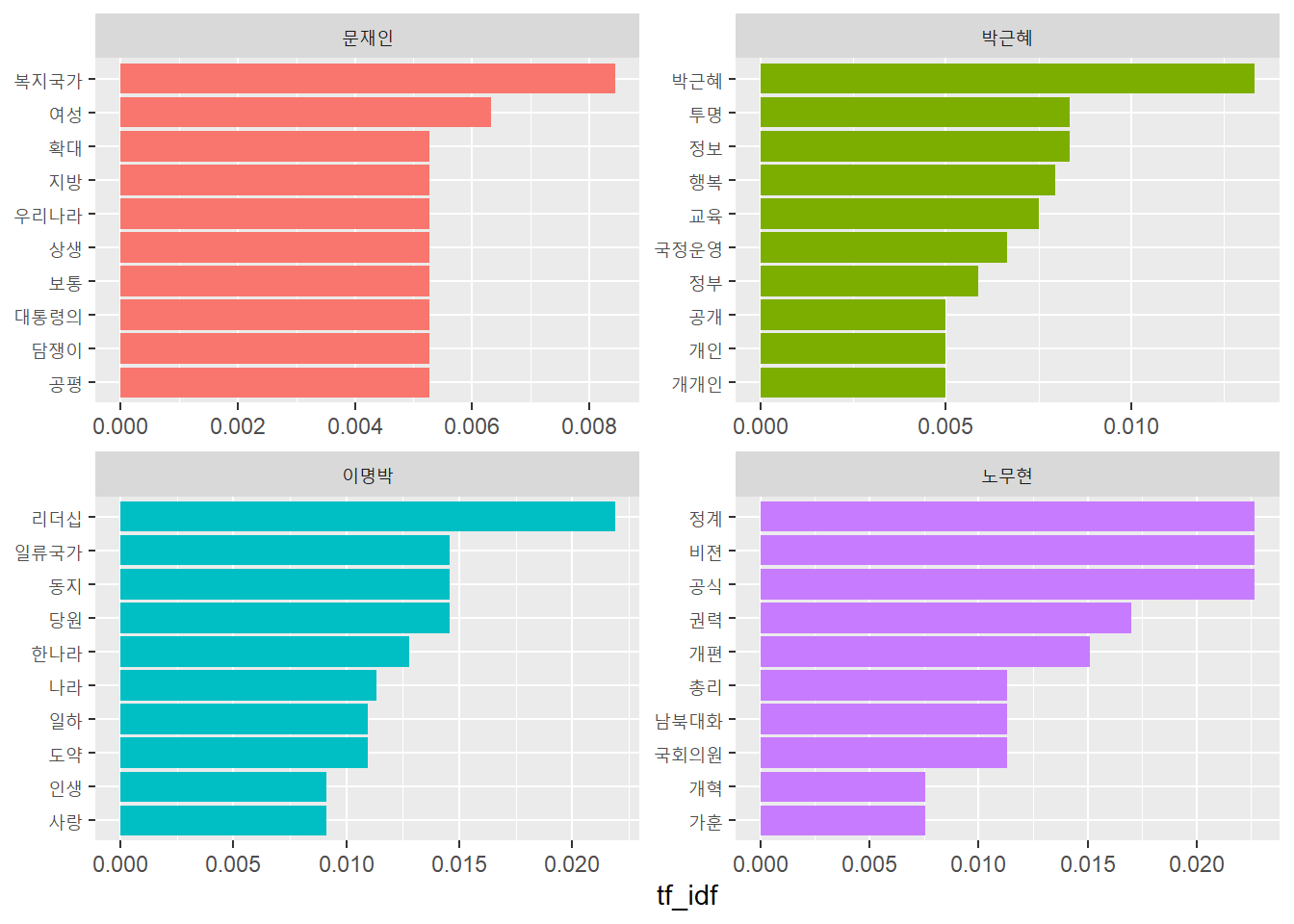
# TF-IDF 구하기
library(tidytext)
frequecy <- frequecy %>%
  bind_tf_idf(term = word, # 단어
              document = president, # 텍스트 구분 기준
              n = n) %>% # 단어 빈도
  arrange(-tf_idf)
frequecy

# A tibble: 1,513 × 6
   president word         n      tf   idf tf_idf
   <chr>     <chr>    <int>   <dbl> <dbl>  <dbl>
 1 노무현    공식         6 0.0163  1.39  0.0227
 2 노무현    비젼         6 0.0163  1.39  0.0227
 3 노무현    정계         6 0.0163  1.39  0.0227
 4 이명박    리더십       6 0.0158  1.39  0.0219
 5 노무현    권력         9 0.0245  0.693 0.0170
 6 노무현    개편         4 0.0109  1.39  0.0151
 7 이명박    당원         4 0.0105  1.39  0.0146
 8 이명박    동지         4 0.0105  1.39  0.0146
 9 이명박    일류국가     4 0.0105  1.39  0.0146
10 박근혜    박근혜       8 0.00962 1.39  0.0133
# ℹ 1,503 more rows

# TF-IDF가 높은 단어 살펴보기
frequecy %>% filter(president == "문재인")

# A tibble: 688 × 6
   president word         n      tf   idf  tf_idf
   <chr>     <chr>    <int>   <dbl> <dbl>   <dbl>
 1 문재인    복지국가     8 0.00608 1.39  0.00843
 2 문재인    여성         6 0.00456 1.39  0.00633
 3 문재인    공평         5 0.00380 1.39  0.00527
 4 문재인    담쟁이       5 0.00380 1.39  0.00527
 5 문재인    대통령의     5 0.00380 1.39  0.00527
 6 문재인    보통         5 0.00380 1.39  0.00527
 7 문재인    상생         5 0.00380 1.39  0.00527
 8 문재인    우리나라    10 0.00760 0.693 0.00527
 9 문재인    지방         5 0.00380 1.39  0.00527
10 문재인    확대        10 0.00760 0.693 0.00527
# ℹ 678 more rows

frequecy %>% filter(president == "박근혜")

# A tibble: 407 × 6
   president word         n      tf   idf  tf_idf
   <chr>     <chr>    <int>   <dbl> <dbl>   <dbl>
 1 박근혜    박근혜       8 0.00962 1.39  0.0133 
 2 박근혜    정보         5 0.00601 1.39  0.00833
 3 박근혜    투명         5 0.00601 1.39  0.00833
 4 박근혜    행복        23 0.0276  0.288 0.00795
 5 박근혜    교육         9 0.0108  0.693 0.00750
 6 박근혜    국정운영     4 0.00481 1.39  0.00666
 7 박근혜    정부        17 0.0204  0.288 0.00588
 8 박근혜    개개인       3 0.00361 1.39  0.00500
 9 박근혜    개인         3 0.00361 1.39  0.00500
10 박근혜    공개         3 0.00361 1.39  0.00500
# ℹ 397 more rows

frequecy %>% filter(president == "이명박")

# A tibble: 202 × 6
   president word         n      tf   idf  tf_idf
   <chr>     <chr>    <int>   <dbl> <dbl>   <dbl>
 1 이명박    리더십       6 0.0158  1.39  0.0219 
 2 이명박    당원         4 0.0105  1.39  0.0146 
 3 이명박    동지         4 0.0105  1.39  0.0146 
 4 이명박    일류국가     4 0.0105  1.39  0.0146 
 5 이명박    한나라       7 0.0184  0.693 0.0128 
 6 이명박    나라        15 0.0395  0.288 0.0114 
 7 이명박    도약         3 0.00789 1.39  0.0109 
 8 이명박    일하         3 0.00789 1.39  0.0109 
 9 이명박    사랑         5 0.0132  0.693 0.00912
10 이명박    인생         5 0.0132  0.693 0.00912
# ℹ 192 more rows

frequecy %>% filter(president == "노무현")

# A tibble: 216 × 6
   president word         n      tf   idf  tf_idf
   <chr>     <chr>    <int>   <dbl> <dbl>   <dbl>
 1 노무현    공식         6 0.0163  1.39  0.0227 
 2 노무현    비젼         6 0.0163  1.39  0.0227 
 3 노무현    정계         6 0.0163  1.39  0.0227 
 4 노무현    권력         9 0.0245  0.693 0.0170 
 5 노무현    개편         4 0.0109  1.39  0.0151 
 6 노무현    국회의원     3 0.00817 1.39  0.0113 
 7 노무현    남북대화     3 0.00817 1.39  0.0113 
 8 노무현    총리         3 0.00817 1.39  0.0113 
 9 노무현    가훈         2 0.00545 1.39  0.00755
10 노무현    개혁         4 0.0109  0.693 0.00755
# ℹ 206 more rows

# TF-IDF가 낮은 단어 살펴보기, 4개가 동일한 값으로 출력됨
frequecy %>%
  filter(president == "문재인") %>%
  arrange(tf_idf)

# A tibble: 688 × 6
   president word       n       tf   idf tf_idf
   <chr>     <chr>  <int>    <dbl> <dbl>  <dbl>
 1 문재인    경쟁       6 0.00456      0      0
 2 문재인    경제      15 0.0114       0      0
 3 문재인    고통       4 0.00304      0      0
 4 문재인    과거       1 0.000760     0      0
 5 문재인    국민      21 0.0160       0      0
 6 문재인    기회       5 0.00380      0      0
 7 문재인    대통령    12 0.00913      0      0
 8 문재인    동안       2 0.00152      0      0
 9 문재인    들이       9 0.00684      0      0
10 문재인    마음       2 0.00152      0      0
# ℹ 678 more rows

frequecy %>%
  filter(president == "박근혜") %>%
  arrange(tf_idf)

# A tibble: 407 × 6
   president word       n      tf   idf tf_idf
   <chr>     <chr>  <int>   <dbl> <dbl>  <dbl>
 1 박근혜    경쟁       1 0.00120     0      0
 2 박근혜    경제      15 0.0180      0      0
 3 박근혜    고통       4 0.00481     0      0
 4 박근혜    과거       2 0.00240     0      0
 5 박근혜    국민      72 0.0865      0      0
 6 박근혜    기회       1 0.00120     0      0
 7 박근혜    대통령     3 0.00361     0      0
 8 박근혜    동안       3 0.00361     0      0
 9 박근혜    들이       3 0.00361     0      0
10 박근혜    마음       3 0.00361     0      0
# ℹ 397 more rows

frequecy %>%
  filter(president == "이명박") %>%
  arrange(tf_idf)

# A tibble: 202 × 6
   president word       n      tf   idf tf_idf
   <chr>     <chr>  <int>   <dbl> <dbl>  <dbl>
 1 이명박    경쟁       3 0.00789     0      0
 2 이명박    경제       5 0.0132      0      0
 3 이명박    고통       1 0.00263     0      0
 4 이명박    과거       1 0.00263     0      0
 5 이명박    국민      13 0.0342      0      0
 6 이명박    기회       3 0.00789     0      0
 7 이명박    대통령     4 0.0105      0      0
 8 이명박    동안       1 0.00263     0      0
 9 이명박    들이       1 0.00263     0      0
10 이명박    마음       1 0.00263     0      0
# ℹ 192 more rows

frequecy %>%
  filter(president == "노무현") %>%
  arrange(tf_idf)

# A tibble: 216 × 6
   president word       n      tf   idf tf_idf
   <chr>     <chr>  <int>   <dbl> <dbl>  <dbl>
 1 노무현    경쟁       1 0.00272     0      0
 2 노무현    경제       1 0.00272     0      0
 3 노무현    고통       1 0.00272     0      0
 4 노무현    과거       1 0.00272     0      0
 5 노무현    국민       7 0.0191      0      0
 6 노무현    기회       1 0.00272     0      0
 7 노무현    대통령     6 0.0163      0      0
 8 노무현    동안       2 0.00545     0      0
 9 노무현    들이       4 0.0109      0      0
10 노무현    마음       1 0.00272     0      0
# ℹ 206 more rows

# 막대 그래프 만들기
# 주요 단어 추출
top10 <- frequecy %>%
  group_by(president) %>%
  slice_max(tf_idf, n = 10, with_ties = F)
top10

# A tibble: 40 × 6
# Groups:   president [4]
   president word         n      tf   idf  tf_idf
   <chr>     <chr>    <int>   <dbl> <dbl>   <dbl>
 1 노무현    공식         6 0.0163  1.39  0.0227 
 2 노무현    비젼         6 0.0163  1.39  0.0227 
 3 노무현    정계         6 0.0163  1.39  0.0227 
 4 노무현    권력         9 0.0245  0.693 0.0170 
 5 노무현    개편         4 0.0109  1.39  0.0151 
 6 노무현    국회의원     3 0.00817 1.39  0.0113 
 7 노무현    남북대화     3 0.00817 1.39  0.0113 
 8 노무현    총리         3 0.00817 1.39  0.0113 
 9 노무현    가훈         2 0.00545 1.39  0.00755
10 노무현    개혁         4 0.0109  0.693 0.00755
# ℹ 30 more rows

# 그래프 순서 정하기
top10$president <- factor(top10$president,
                          levels = c("문재인", "박근혜", "이명박", "노무현"))

# 막대 그래프 만들기
library(ggplot2)
library(showtext)

Loading required package: sysfonts

Loading required package: showtextdb

ggplot(top10, aes(x = reorder_within(word, tf_idf, president),
                  y = tf_idf,
                  fill = president)) +
  geom_col(show.legend = F) +
  coord_flip() +
  facet_wrap(~ president, scales = "free", ncol = 2) +
  scale_x_reordered() +
  labs(x = NULL)

Sentimental Analysis

군산대 감성사전 csv

# 감정 사전 불러오기
dic <- read_csv('data/knu_sentiment_lexicon.csv')

Rows: 14854 Columns: 2
── Column specification ────────────────────────────────────────────────────────
Delimiter: ","
chr (1): word
dbl (1): polarity

ℹ Use `spec()` to retrieve the full column specification for this data.
ℹ Specify the column types or set `show_col_types = FALSE` to quiet this message.

# 긍정 단어
dic %>%
  filter(polarity == 2) %>%
  arrange(word)

# A tibble: 2,602 × 2
   word              polarity
   <chr>                <dbl>
 1 가능성이 늘어나다        2
 2 가능성이 있다고          2
 3 가능하다                 2
 4 가볍고 상쾌하다          2
 5 가볍고 상쾌한            2
 6 가볍고 시원하게          2
 7 가볍고 편안하게          2
 8 가볍고 환하게            2
 9 가운데에서 뛰어남        2
10 가장 거룩한              2
# ℹ 2,592 more rows

# 부정 단어
dic %>%
  filter(polarity == -2) %>%
  arrange(word)

# A tibble: 4,799 × 2
   word            polarity
   <chr>              <dbl>
 1 가난                  -2
 2 가난뱅이              -2
 3 가난살이              -2
 4 가난살이하다          -2
 5 가난설음              -2
 6 가난에                -2
 7 가난에 쪼들려서       -2
 8 가난하게              -2
 9 가난하고              -2
10 가난하고 어렵다       -2
# ℹ 4,789 more rows

# 감정 단어의 종류 살펴보기
dic %>%
  filter(word %in% c("좋은", "나쁜"))

# A tibble: 2 × 2
  word  polarity
  <chr>    <dbl>
1 좋은         2
2 나쁜        -2

dic %>%
  filter(word %in% c("기쁜", "슬픈"))

# A tibble: 2 × 2
  word  polarity
  <chr>    <dbl>
1 슬픈        -2
2 기쁜         2

# 이모티콘
library(stringr)
dic %>%
  filter(!str_detect(word, "[가-힣]")) %>%
  arrange(word)

# A tibble: 77 × 2
   word  polarity
   <chr>    <dbl>
 1 (-;          1
 2 (-_-)       -1
 3 (;_;)       -1
 4 (T_T)       -1
 5 (^-^)        1
 6 (^^)         1
 7 (^^*         1
 8 (^_^)        1
 9 (^_^;       -1
10 (^o^)        1
# ℹ 67 more rows

# 총 14,854개 단어
dic %>%
  mutate(sentiment = ifelse(polarity >= 1, "pos",
                            ifelse(polarity <= -1, "neg", "neu"))) %>%
  count(sentiment)

# A tibble: 3 × 2
  sentiment     n
  <chr>     <int>
1 neg        9829
2 neu         154
3 pos        4871

# 문장의 감정 점수 구하기
# 1. 단어 기준으로 토큰화하기
df <- tibble(sentence = c("디자인 예쁘고 마감도 좋아서 만족스럽다.",
                          "디자인은 괜찮다. 그런데 마감이 나쁘고 가격도 비싸다."))

library(tidytext)
df <- df %>%
  unnest_tokens(input = sentence,
                output = word,
                token = "words",
                drop = F)
df

# A tibble: 12 × 2
   sentence                                             word      
   <chr>                                                <chr>     
 1 디자인 예쁘고 마감도 좋아서 만족스럽다.              디자인    
 2 디자인 예쁘고 마감도 좋아서 만족스럽다.              예쁘고    
 3 디자인 예쁘고 마감도 좋아서 만족스럽다.              마감도    
 4 디자인 예쁘고 마감도 좋아서 만족스럽다.              좋아서    
 5 디자인 예쁘고 마감도 좋아서 만족스럽다.              만족스럽다
 6 디자인은 괜찮다. 그런데 마감이 나쁘고 가격도 비싸다. 디자인은  
 7 디자인은 괜찮다. 그런데 마감이 나쁘고 가격도 비싸다. 괜찮다    
 8 디자인은 괜찮다. 그런데 마감이 나쁘고 가격도 비싸다. 그런데    
 9 디자인은 괜찮다. 그런데 마감이 나쁘고 가격도 비싸다. 마감이    
10 디자인은 괜찮다. 그런데 마감이 나쁘고 가격도 비싸다. 나쁘고    
11 디자인은 괜찮다. 그런데 마감이 나쁘고 가격도 비싸다. 가격도    
12 디자인은 괜찮다. 그런데 마감이 나쁘고 가격도 비싸다. 비싸다    

# 2. 단어에 감정 점수 부여하기
df <- df %>%
  left_join(dic, by = "word") %>%
  mutate(polarity = ifelse(is.na(polarity), 0, polarity))
df

# A tibble: 12 × 3
   sentence                                             word       polarity
   <chr>                                                <chr>         <dbl>
 1 디자인 예쁘고 마감도 좋아서 만족스럽다.              디자인            0
 2 디자인 예쁘고 마감도 좋아서 만족스럽다.              예쁘고            2
 3 디자인 예쁘고 마감도 좋아서 만족스럽다.              마감도            0
 4 디자인 예쁘고 마감도 좋아서 만족스럽다.              좋아서            2
 5 디자인 예쁘고 마감도 좋아서 만족스럽다.              만족스럽다        2
 6 디자인은 괜찮다. 그런데 마감이 나쁘고 가격도 비싸다. 디자인은          0
 7 디자인은 괜찮다. 그런데 마감이 나쁘고 가격도 비싸다. 괜찮다            1
 8 디자인은 괜찮다. 그런데 마감이 나쁘고 가격도 비싸다. 그런데            0
 9 디자인은 괜찮다. 그런데 마감이 나쁘고 가격도 비싸다. 마감이            0
10 디자인은 괜찮다. 그런데 마감이 나쁘고 가격도 비싸다. 나쁘고           -2
11 디자인은 괜찮다. 그런데 마감이 나쁘고 가격도 비싸다. 가격도            0
12 디자인은 괜찮다. 그런데 마감이 나쁘고 가격도 비싸다. 비싸다           -2

# 3. 문장별로 감정 점수 합산하기
score_df <- df %>%
  group_by(sentence) %>%
  summarise(score = sum(polarity))
score_df

# A tibble: 2 × 2
  sentence                                             score
  <chr>                                                <dbl>
1 디자인 예쁘고 마감도 좋아서 만족스럽다.                  6
2 디자인은 괜찮다. 그런데 마감이 나쁘고 가격도 비싸다.    -3

Sentimental Analysis for the comments

댓글 감성 분석

# 데이터 불러오기
raw_news_comment <- read_csv("data/news_comment_parasite.csv")

Rows: 4150 Columns: 5
── Column specification ────────────────────────────────────────────────────────
Delimiter: ","
chr  (4): reply, press, title, url
dttm (1): reg_time

ℹ Use `spec()` to retrieve the full column specification for this data.
ℹ Specify the column types or set `show_col_types = FALSE` to quiet this message.

raw_news_comment

# A tibble: 4,150 × 5
   reg_time            reply                                   press title url  
   <dttm>              <chr>                                   <chr> <chr> <chr>
 1 2020-02-10 16:59:02 "정말 우리 집에 좋은 일이 생겨 기쁘고 … MBC   '기…  http…
 2 2020-02-10 13:32:24 "와 너무 기쁘다! 이 시국에 정말 내 일…  SBS   [영…  http…
 3 2020-02-10 12:30:09 "우리나라의 영화감독분들 그리고 앞으로… 한겨… ‘기…  http…
 4 2020-02-10 13:08:22 "봉준호 감독과 우리나라 대한민국 모두 … 한겨… ‘기…  http…
 5 2020-02-10 16:25:41 "노벨상 탄느낌이네요\r\n축하축하 합니…  한겨… ‘기…  http…
 6 2020-02-10 12:31:45 "기생충 상 받을때 박수 쳤어요.감독상도… 한겨… ‘기…  http…
 7 2020-02-10 12:31:33 "대한민국 영화사를 새로 쓰고 계시네요 … 한겨… ‘기…  http…
 8 2020-02-11 09:20:52 "저런게 아카데미상 받으면  '태극기 휘…  한겨… ‘기…  http…
 9 2020-02-10 20:53:27 "다시한번 보여주세요 영화관에서 보고싶… 한겨… ‘기…  http…
10 2020-02-10 20:22:41 "대한민국 BTS와함께  봉준호감독님까지\… 한겨… ‘기…  http…
# ℹ 4,140 more rows

# 기본적인 전처리
library(textclean)
news_comment <- raw_news_comment %>%
  mutate(id = row_number(),
         reply = str_squish(replace_html(reply)))
news_comment

# A tibble: 4,150 × 6
   reg_time            reply                             press title url      id
   <dttm>              <chr>                             <chr> <chr> <chr> <int>
 1 2020-02-10 16:59:02 정말 우리 집에 좋은 일이 생겨 기… MBC   '기…  http…     1
 2 2020-02-10 13:32:24 와 너무 기쁘다! 이 시국에 정말 …  SBS   [영…  http…     2
 3 2020-02-10 12:30:09 우리나라의 영화감독분들 그리고 …  한겨… ‘기…  http…     3
 4 2020-02-10 13:08:22 봉준호 감독과 우리나라 대한민국 … 한겨… ‘기…  http…     4
 5 2020-02-10 16:25:41 노벨상 탄느낌이네요 축하축하 합…  한겨… ‘기…  http…     5
 6 2020-02-10 12:31:45 기생충 상 받을때 박수 쳤어요.감…  한겨… ‘기…  http…     6
 7 2020-02-10 12:31:33 대한민국 영화사를 새로 쓰고 계시… 한겨… ‘기…  http…     7
 8 2020-02-11 09:20:52 저런게 아카데미상 받으면 '태극기… 한겨… ‘기…  http…     8
 9 2020-02-10 20:53:27 다시한번 보여주세요 영화관에서 …  한겨… ‘기…  http…     9
10 2020-02-10 20:22:41 대한민국 BTS와함께 봉준호감독님…  한겨… ‘기…  http…    10
# ℹ 4,140 more rows

# 데이터 구조 확인
glimpse(news_comment)

Rows: 4,150
Columns: 6
$ reg_time <dttm> 2020-02-10 16:59:02, 2020-02-10 13:32:24, 2020-02-10 12:30:0…
$ reply    <chr> "정말 우리 집에 좋은 일이 생겨 기쁘고 행복한 것처럼!! 나의 일…
$ press    <chr> "MBC", "SBS", "한겨레", "한겨레", "한겨레", "한겨레", "한겨레…
$ title    <chr> "'기생충' 아카데미 작품상까지 4관왕…영화사 새로 썼다", "[영상…
$ url      <chr> "https://news.naver.com/main/read.nhn?mode=LSD&mid=sec&sid1=1…
$ id       <int> 1, 2, 3, 4, 5, 6, 7, 8, 9, 10, 11, 12, 13, 14, 15, 16, 17, 18…

# 단어 기준으로 토큰화하고 감정 점수 부여하기
# 토큰화
word_comment <- news_comment %>%
  unnest_tokens(input = reply,
                output = word,
                token = "words",
                drop = F)

word_comment %>%
  select(word, reply)

# A tibble: 37,718 × 2
   word   reply                                                                
   <chr>  <chr>                                                                
 1 정말   정말 우리 집에 좋은 일이 생겨 기쁘고 행복한 것처럼!! 나의 일인 양 행…
 2 우리   정말 우리 집에 좋은 일이 생겨 기쁘고 행복한 것처럼!! 나의 일인 양 행…
 3 집에   정말 우리 집에 좋은 일이 생겨 기쁘고 행복한 것처럼!! 나의 일인 양 행…
 4 좋은   정말 우리 집에 좋은 일이 생겨 기쁘고 행복한 것처럼!! 나의 일인 양 행…
 5 일이   정말 우리 집에 좋은 일이 생겨 기쁘고 행복한 것처럼!! 나의 일인 양 행…
 6 생겨   정말 우리 집에 좋은 일이 생겨 기쁘고 행복한 것처럼!! 나의 일인 양 행…
 7 기쁘고 정말 우리 집에 좋은 일이 생겨 기쁘고 행복한 것처럼!! 나의 일인 양 행…
 8 행복한 정말 우리 집에 좋은 일이 생겨 기쁘고 행복한 것처럼!! 나의 일인 양 행…
 9 것처럼 정말 우리 집에 좋은 일이 생겨 기쁘고 행복한 것처럼!! 나의 일인 양 행…
10 나의   정말 우리 집에 좋은 일이 생겨 기쁘고 행복한 것처럼!! 나의 일인 양 행…
# ℹ 37,708 more rows

# 감정 점수 부여
word_comment <- word_comment %>%
  left_join(dic, by = "word") %>%
  mutate(polarity = ifelse(is.na(polarity), 0, polarity))

word_comment %>%
  select(word, polarity)

# A tibble: 37,718 × 2
   word   polarity
   <chr>     <dbl>
 1 정말          0
 2 우리          0
 3 집에          0
 4 좋은          2
 5 일이          0
 6 생겨          0
 7 기쁘고        2
 8 행복한        2
 9 것처럼        0
10 나의          0
# ℹ 37,708 more rows

# 자주 사용된 감정 단어 살펴보기
# 1. 감정 분류하기
word_comment <- word_comment %>%
  mutate(sentiment = ifelse(polarity == 2, "pos",
                            ifelse(polarity == -2, "neg", "neu")))

word_comment %>%
  count(sentiment)

# A tibble: 3 × 2
  sentiment     n
  <chr>     <int>
1 neg         285
2 neu       36671
3 pos         762

# 2. 막대 그래프 만들기
top10_sentiment <- word_comment %>%
  filter(sentiment != "neu") %>%
  count(sentiment, word) %>%
  group_by(sentiment) %>%
  slice_max(n, n = 10)

top10_sentiment

# A tibble: 22 × 3
# Groups:   sentiment [2]
   sentiment word       n
   <chr>     <chr>  <int>
 1 neg       소름      56
 2 neg       소름이    16
 3 neg       아니다    15
 4 neg       우울한     9
 5 neg       해         8
 6 neg       미친       7
 7 neg       가난한     5
 8 neg       어려운     5
 9 neg       힘든       5
10 neg       더러운     4
# ℹ 12 more rows

ggplot(top10_sentiment, aes(x = reorder(word, n),
                            y = n,
                            fill = sentiment)) +
  geom_col() +
  coord_flip() +
  geom_text(aes(label = n), hjust = -0.3) +
  facet_wrap(~ sentiment, scales = "free") +
  scale_y_continuous(expand = expansion(mult = c(0.05, 0.15))) +
  labs(x = NULL) 

댓글별 감정 점수 구하고 댓글 살펴보기

# 1. 댓글별 감정 점수 구하기
score_comment <- word_comment %>%
  group_by(id, reply) %>%
  summarise(score = sum(polarity)) %>%
  ungroup()

`summarise()` has grouped output by 'id'. You can override using the `.groups`
argument.

score_comment %>%
  select(score, reply)

# A tibble: 4,140 × 2
   score reply                                                                  
   <dbl> <chr>                                                                  
 1     6 정말 우리 집에 좋은 일이 생겨 기쁘고 행복한 것처럼!! 나의 일인 양 행복…
 2     6 와 너무 기쁘다! 이 시국에 정말 내 일같이 기쁘고 감사하다!!! 축하드려요…
 3     4 우리나라의 영화감독분들 그리고 앞으로 그 꿈을 그리는 분들에게 큰 영감… 
 4     3 봉준호 감독과 우리나라 대한민국 모두 자랑스럽다. 세계 어디를 가고 우리…
 5     0 노벨상 탄느낌이네요 축하축하 합니다                                    
 6     0 기생충 상 받을때 박수 쳤어요.감독상도 기대해요.봉준호 감독 화이팅^^    
 7     0 대한민국 영화사를 새로 쓰고 계시네요 ㅊㅊㅊ                            
 8     0 저런게 아카데미상 받으면 '태극기 휘날리며'' '광해' '명량''은 전부문 휩…
 9     0 다시한번 보여주세요 영화관에서 보고싶은디                              
10     2 대한민국 BTS와함께 봉준호감독님까지 대단하고 한국의 문화에 자긍심을 가…
# ℹ 4,130 more rows

# 2. 감정 점수 높은 댓글 살펴보기
# 긍정 댓글
score_comment %>%
  select(score, reply) %>%
  arrange(-score)

# A tibble: 4,140 × 2
   score reply                                                                  
   <dbl> <chr>                                                                  
 1    11 아니 다른상을 받은것도 충분히 대단하고 굉장하지만 최고의 영예인 작품상…
 2     9 봉준호의 위대한 업적은 진보 영화계의 위대한 업적이고 대한민국의 업적입…
 3     7 이 수상소식을 듣고 억수로 기뻐하는 가족이 있을것 같다. SNS를 통해 자기…
 4     7 감사 감사 감사 수상 소감도 3관왕 답네요                                
 5     6 정말 우리 집에 좋은 일이 생겨 기쁘고 행복한 것처럼!! 나의 일인 양 행복…
 6     6 와 너무 기쁘다! 이 시국에 정말 내 일같이 기쁘고 감사하다!!! 축하드려요…
 7     6 축하 축하 축하 모두들 수고 하셨어요 기생충 화이팅                      
 8     6 축하!!!! 축하!!!!! 오스카의 정복은 무엇보다 시나리오의 힘이다. 작가의 …
 9     6 조여정 ㆍ예쁜얼굴때문에 연기력을 제대로 평가받지 못해 안타깝던 내가 좋…
10     6 좋은 걸 좋다고 말하지 못하는 인간들이 참 불쌍해지네....댓글 보니 인생… 
# ℹ 4,130 more rows

# 부정 댓글
score_comment %>%
  select(score, reply) %>%
  arrange(score)

# A tibble: 4,140 × 2
   score reply                                                                  
   <dbl> <chr>                                                                  
 1    -7 기생충 영화 한국인 으로써 싫다 대단히 싫다!! 가난한 서민들의 마지막 자…
 2    -6 이 페미민국이 잘 되는 게 아주 싫다. 최악의 나쁜일들과 불운, 불행, 어둡…
 3    -5 특정 인물의 성공을 국가의 부흥으로 연관짓는 것은 미개한 발상이다. 봉준…
 4    -4 좌파들이 나라 망신 다 시킨다..ㅠ 설레발 오지게 치더니..꼴랑 각본상 하… 
 5    -4 부패한 386 민주화 세대 정권의 무분별한 포퓰리즘으로 탄생한 좀비들의 살…
 6    -4 기생충 내용은 좋은데 제목이 그래요. 극 중 송강호가족이 부잣집에 대해서…
 7    -4 이런 감독과 이런 배우보고 좌좀 이라고 지1랄하던 그분들 다 어디계시냐? …
 8    -4 축하합니다. 근데 현실 세계인 한국에선 그보다 훨씬 나쁜 넘인 조로남불 … 
 9    -4 큰일이다....국제적 망신이다...전 세계사람들이 우리나라를 기생충으로 보…
10    -4 더럽고 추잡한 그들만의 리그                                            
# ℹ 4,130 more rows

# 감정 경향 살펴보기
# 1. 감정 점수 빈도 구하기
score_comment %>%
  count(score)

# A tibble: 17 × 2
   score     n
   <dbl> <int>
 1    -7     1
 2    -6     1
 3    -5     1
 4    -4    17
 5    -3    35
 6    -2   175
 7    -1   206
 8     0  2897
 9     1   222
10     2   432
11     3    57
12     4    71
13     5     7
14     6    14
15     7     2
16     9     1
17    11     1

# 2. 감정 분류하고 막대 그래프 만들기
# 감정 분류하기
score_comment <- score_comment %>%
  mutate(sentiment = ifelse(score >= 1, "pos",
                            ifelse(score <= -1, "neg", "neu")))

# 감정 빈도와 비율 구하기
frequency_score <- score_comment %>%
  count(sentiment) %>%
  mutate(ratio = n/sum(n)*100)
frequency_score

# A tibble: 3 × 3
  sentiment     n ratio
  <chr>     <int> <dbl>
1 neg         436  10.5
2 neu        2897  70.0
3 pos         807  19.5

# 막대 그래프 만들기
ggplot(frequency_score, aes(x = sentiment, y = n, fill = sentiment)) +
  geom_col() +
  geom_text(aes(label = n), vjust = -0.3) +
  scale_x_discrete(limits = c("pos", "neu", "neg"))

# 3. 비율 누적 막대 그래프 만들기
df <- tibble(contry = c("Korea", "Korea", "Japen", "Japen"), # 축
             sex = c("M", "F", "M", "F"), # 누적 막대
             ratio = c(60, 40, 30, 70)) # 값
df

# A tibble: 4 × 3
  contry sex   ratio
  <chr>  <chr> <dbl>
1 Korea  M        60
2 Korea  F        40
3 Japen  M        30
4 Japen  F        70

ggplot(df, aes(x = contry, y = ratio, fill = sex)) + geom_col()

ggplot(df, aes(x = contry, y = ratio, fill = sex)) +
  geom_col() +
  geom_text(aes(label = paste0(ratio, "%")), # % 표시
            position = position_stack(vjust = 0.5)) # 가운데 표시

# 댓글의 감정 비율로 누적 막대 그래프 만들기
# 더미 변수 생성
frequency_score$dummy <- 0
frequency_score

# A tibble: 3 × 4
  sentiment     n ratio dummy
  <chr>     <int> <dbl> <dbl>
1 neg         436  10.5     0
2 neu        2897  70.0     0
3 pos         807  19.5     0

ggplot(frequency_score, aes(x = dummy, y = ratio, fill = sentiment)) +
  geom_col() +
  geom_text(aes(label = paste0(round(ratio, 1), "%")),
            position = position_stack(vjust = 0.5)) +
  theme(axis.title.x = element_blank(), # x축 이름 삭제
        axis.text.x = element_blank(), # x축 값 삭제
        axis.ticks.x = element_blank()) # x축 눈금 삭제

Word Frequency by Sentiment Category

감정 범주별 단어 빈도

# 감정 범주별 단어 빈도 구하기
# 1. 토큰화하고 두 글자 이상 한글 단어만 남기기
comment <- score_comment %>%
  unnest_tokens(input = reply, # 단어 기준 토큰화
                output = word,
                token = "words",
                drop = F) %>%
  filter(str_detect(word, "[가-힣]") & # 한글 추출
           str_count(word) >= 2) # 두 글자 이상 추출

# 2. 감정 범주별 빈도 구하기
frequency_word <- comment %>%
  filter(str_count(word) >= 2) %>%
  count(sentiment, word, sort = T)
frequency_word

# A tibble: 19,223 × 3
   sentiment word               n
   <chr>     <chr>          <int>
 1 neu       축하합니다       214
 2 neu       봉준호           203
 3 neu       기생충           164
 4 neu       축하드립니다     155
 5 neu       정말             146
 6 neu       대박             134
 7 neu       진짜             121
 8 pos       봉준호           106
 9 pos       정말              97
10 neu       자랑스럽습니다    96
# ℹ 19,213 more rows

# 긍정 댓글 고빈도 단어
frequency_word %>%
  filter(sentiment == "pos")

# A tibble: 5,234 × 3
   sentiment word           n
   <chr>     <chr>      <int>
 1 pos       봉준호       106
 2 pos       정말          97
 3 pos       대단하다      83
 4 pos       진짜          79
 5 pos       자랑스럽다    78
 6 pos       축하          63
 7 pos       대한민국      61
 8 pos       영화          58
 9 pos       멋지다        55
10 pos       기생충        53
# ℹ 5,224 more rows

# 부정 댓글 고빈도 단어
frequency_word %>%
  filter(sentiment == "neg")

# A tibble: 4,080 × 3
   sentiment word             n
   <chr>     <chr>        <int>
 1 neg       소름            49
 2 neg       봉준호          47
 3 neg       기생충          33
 4 neg       이런            33
 5 neg       정말            32
 6 neg       진짜            26
 7 neg       좌빨            21
 8 neg       너무            20
 9 neg       블랙리스트에    19
10 neg       영화            18
# ℹ 4,070 more rows

# 상대적으로 자주 사용된 단어 비교하기
# 1. 로그 오즈비 구하기
# wide form으로 변환
comment_wide <- frequency_word %>%
  filter(sentiment != "neu") %>%
  pivot_wider(names_from = sentiment,
              values_from = n,
              values_fill = list(n = 0))
comment_wide

# A tibble: 8,380 × 3
   word         pos   neg
   <chr>      <int> <int>
 1 봉준호       106    47
 2 정말          97    32
 3 대단하다      83     1
 4 진짜          79    26
 5 자랑스럽다    78     1
 6 축하          63     0
 7 대한민국      61     4
 8 영화          58    18
 9 멋지다        55     0
10 기생충        53    33
# ℹ 8,370 more rows

# 로그 오즈비 구하기
comment_wide <- comment_wide %>%
  mutate(log_odds_ratio = log(((pos + 1) / (sum(pos + 1))) /
                                ((neg + 1) / (sum(neg + 1)))))
comment_wide

# A tibble: 8,380 × 4
   word         pos   neg log_odds_ratio
   <chr>      <int> <int>          <dbl>
 1 봉준호       106    47          0.589
 2 정말          97    32          0.876
 3 대단하다      83     1          3.52 
 4 진짜          79    26          0.873
 5 자랑스럽다    78     1          3.46 
 6 축하          63     0          3.95 
 7 대한민국      61     4          2.30 
 8 영화          58    18          0.920
 9 멋지다        55     0          3.81 
10 기생충        53    33          0.250
# ℹ 8,370 more rows

# 2. 로그 오즈비가 가장 큰 단어 10개씩 추출하기
top10 <- comment_wide %>%
  group_by(sentiment = ifelse(log_odds_ratio > 0, "pos", "neg")) %>%
  slice_max(abs(log_odds_ratio), n = 10, with_ties = F)
top10

# A tibble: 20 × 5
# Groups:   sentiment [2]
   word         pos   neg log_odds_ratio sentiment
   <chr>      <int> <int>          <dbl> <chr>    
 1 소름           2    49          -3.03 neg      
 2 좌빨           1    21          -2.61 neg      
 3 못한           0     7          -2.29 neg      
 4 미친           0     7          -2.29 neg      
 5 좌좀           0     6          -2.16 neg      
 6 소름이         1    12          -2.08 neg      
 7 가난한         0     5          -2.00 neg      
 8 모르는         0     5          -2.00 neg      
 9 아쉽다         0     5          -2.00 neg      
10 닭그네         0     4          -1.82 neg      
11 축하          63     0           3.95 pos      
12 멋지다        55     0           3.81 pos      
13 대단한        47     0           3.66 pos      
14 좋은          42     0           3.55 pos      
15 대단하다      83     1           3.52 pos      
16 자랑스럽다    78     1           3.46 pos      
17 최고          27     0           3.12 pos      
18 세계적인      24     0           3.01 pos      
19 최고의        23     0           2.97 pos      
20 위대한        22     0           2.92 pos      

# 3. 막대 그래프 만들기
ggplot(top10, aes(x = reorder(word, log_odds_ratio),
                  y = log_odds_ratio,
                  fill = sentiment)) +
  geom_col() +
  coord_flip() +
  labs(x = NULL)

Modify Emotion Words

감정 단어 수정

# 감정 단어가 사용된 원문 살펴보기
# "소름"이 사용된 댓글
score_comment %>%
  filter(str_detect(reply, "소름")) %>%
  select(reply)

# A tibble: 131 × 1
   reply                                                                       
   <chr>                                                                       
 1 소름돋네요                                                                  
 2 와..진짜소름 저 소리처음질렀어요 눈물나요.. ㅠㅠ                            
 3 생중계 보며 봉준호 할 때 소름이~~~!! ㅠㅠ 수상소감들으며 함께 가슴이 벅차네…
 4 와 보다가 소름 짝 수고들하셨어요                                            
 5 한국어 소감 듣는데 소름돋네 축하드립니다                                    
 6 대단하다!! 봉준호 이름 나오자마자 소름                                      
 7 와우 브라보~ 키아누리브스의 봉준호, 순간 소름이.. 멋지십니다.               
 8 소름 돋네요. 축하합니다                                                     
 9 소름.... 기생충 각본집 산거 다시한번 잘했다는 생각이ㅠㅠㅠ 축하해요!!!!!!   
10 소름끼쳤어요 너무 멋집니다 ^^!!!!                                           
# ℹ 121 more rows

# "미친"이 사용된 댓글
score_comment %>%
  filter(str_detect(reply, "미친")) %>%
  select(reply)

# A tibble: 15 × 1
   reply                                                                        
   <chr>                                                                        
 1 와 3관왕 미친                                                                
 2 미친거야 이건~~                                                              
 3 Korea 대단합니다 김연아 방탄 봉준호 스포츠 음악 영화 못하는게 없어요 좌빨 감…
 4 청룡영화제에서 다른나라가 상을 휩쓴거죠? 와..미쳤다 미국영화제에서 한국이 빅…
 5 설마했는데 감독상, 작품상, 각본상을 죄다 휩쓸어버릴 줄이야. 이건 미친 꿈이야…
 6 완전 완전...미친촌재감~이런게 바로 애국이지~ 존경합니다~                     
 7 이세상엔 참 미 친 인간들이 많다는걸 댓글에서 다시한번 느낀다..모두가 축하해… 
 8 올해 아카데미 최다 수상작이기도 하다 이건 진짜 미친사건이다                  
 9 CJ회장이 저기서 왜 언급되는지... 미친 부회장.. 공과사 구분 못하는 정권의 홍… 
10 미친봉                                                                       
11 미친 3관왕 ㄷㄷㄷㄷㄷ                                                        
12 진짜 미친일...                                                               
13 나도모르게 보다가 육성으로 미친...ㅋㅋㅋㅋ 대박ㅜ                            
14 헐...감독상...미친...미쳤다..소름돋는다...                                   
15 인정할건인정하자 봉감독 송배우 이배우 조배우등 인정하자 또 가로세로 ㅆㄹㄱ들…

dic %>% filter(word %in% c("소름", "소름이", "미친"))

# A tibble: 3 × 2
  word   polarity
  <chr>     <dbl>
1 소름이       -2
2 소름         -2
3 미친         -2

# 감정 사전 수정하기
new_dic <- dic %>%
  mutate(polarity = ifelse(word %in% c("소름", "소름이", "미친"), 2, polarity))
new_dic %>% filter(word %in% c("소름", "소름이", "미친"))

# A tibble: 3 × 2
  word   polarity
  <chr>     <dbl>
1 소름이        2
2 소름          2
3 미친          2

# 수정한 사전으로 감정 점수 부여하기
new_word_comment <- word_comment %>%
  select(-polarity) %>%
  left_join(new_dic, by = "word") %>%
  mutate(polarity = ifelse(is.na(polarity), 0, polarity))

# 댓글별 감정 점수 구하기
new_score_comment <- new_word_comment %>%
  group_by(id, reply) %>%
  summarise(score = sum(polarity)) %>%
  ungroup()

`summarise()` has grouped output by 'id'. You can override using the `.groups`
argument.

new_score_comment %>%
  select(score, reply) %>%
  arrange(-score)

# A tibble: 4,140 × 2
   score reply                                                                  
   <dbl> <chr>                                                                  
 1    11 아니 다른상을 받은것도 충분히 대단하고 굉장하지만 최고의 영예인 작품상…
 2     9 봉준호의 위대한 업적은 진보 영화계의 위대한 업적이고 대한민국의 업적입…
 3     8 소름 소름 진짜 멋지다 대단하다                                         
 4     7 이 수상소식을 듣고 억수로 기뻐하는 가족이 있을것 같다. SNS를 통해 자기…
 5     7 감사 감사 감사 수상 소감도 3관왕 답네요                                
 6     6 정말 우리 집에 좋은 일이 생겨 기쁘고 행복한 것처럼!! 나의 일인 양 행복…
 7     6 와 너무 기쁘다! 이 시국에 정말 내 일같이 기쁘고 감사하다!!! 축하드려요…
 8     6 축하 축하 축하 모두들 수고 하셨어요 기생충 화이팅                      
 9     6 생중계 보며 봉준호 할 때 소름이~~~!! ㅠㅠ 수상소감들으며 함께 가슴이 … 
10     6 축하!!!! 축하!!!!! 오스카의 정복은 무엇보다 시나리오의 힘이다. 작가의 …
# ℹ 4,130 more rows

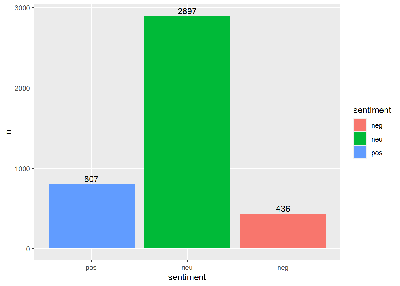
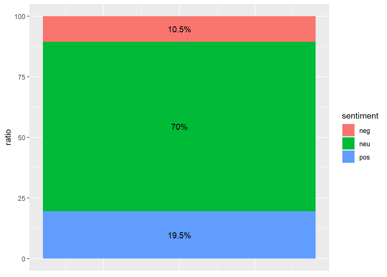
# 전반적인 감정 경향 살펴보기
# 1. 감정 분류하기
# 1점 기준으로 긍정 중립 부정 분류
new_score_comment <- new_score_comment %>%
  mutate(sentiment = ifelse(score >= 1, "pos",
                            ifelse(score <= -1, "neg", "neu")))

# 2. 감정 범주별 빈도와 비율 구하기
# 원본 감정 사전 활용
score_comment %>%
  count(sentiment) %>%
  mutate(ratio = n/sum(n)*100)

# A tibble: 3 × 3
  sentiment     n ratio
  <chr>     <int> <dbl>
1 neg         436  10.5
2 neu        2897  70.0
3 pos         807  19.5

# 수정한 감정 사전 활용
new_score_comment %>%
  count(sentiment) %>%
  mutate(ratio = n/sum(n)*100)

# A tibble: 3 × 3
  sentiment     n ratio
  <chr>     <int> <dbl>
1 neg         368  8.89
2 neu        2890 69.8 
3 pos         882 21.3 

# 3. 분석 결과 비교하기
word <- "소름|소름이|미친"

# 원본 감정 사전 활용
score_comment %>%
  filter(str_detect(reply, word)) %>%
  count(sentiment)

# A tibble: 3 × 2
  sentiment     n
  <chr>     <int>
1 neg          73
2 neu          63
3 pos           9

# 수정한 감정 사전 활용
new_score_comment %>%
  filter(str_detect(reply, word)) %>%
  count(sentiment)

# A tibble: 3 × 2
  sentiment     n
  <chr>     <int>
1 neg           5
2 neu          56
3 pos          84

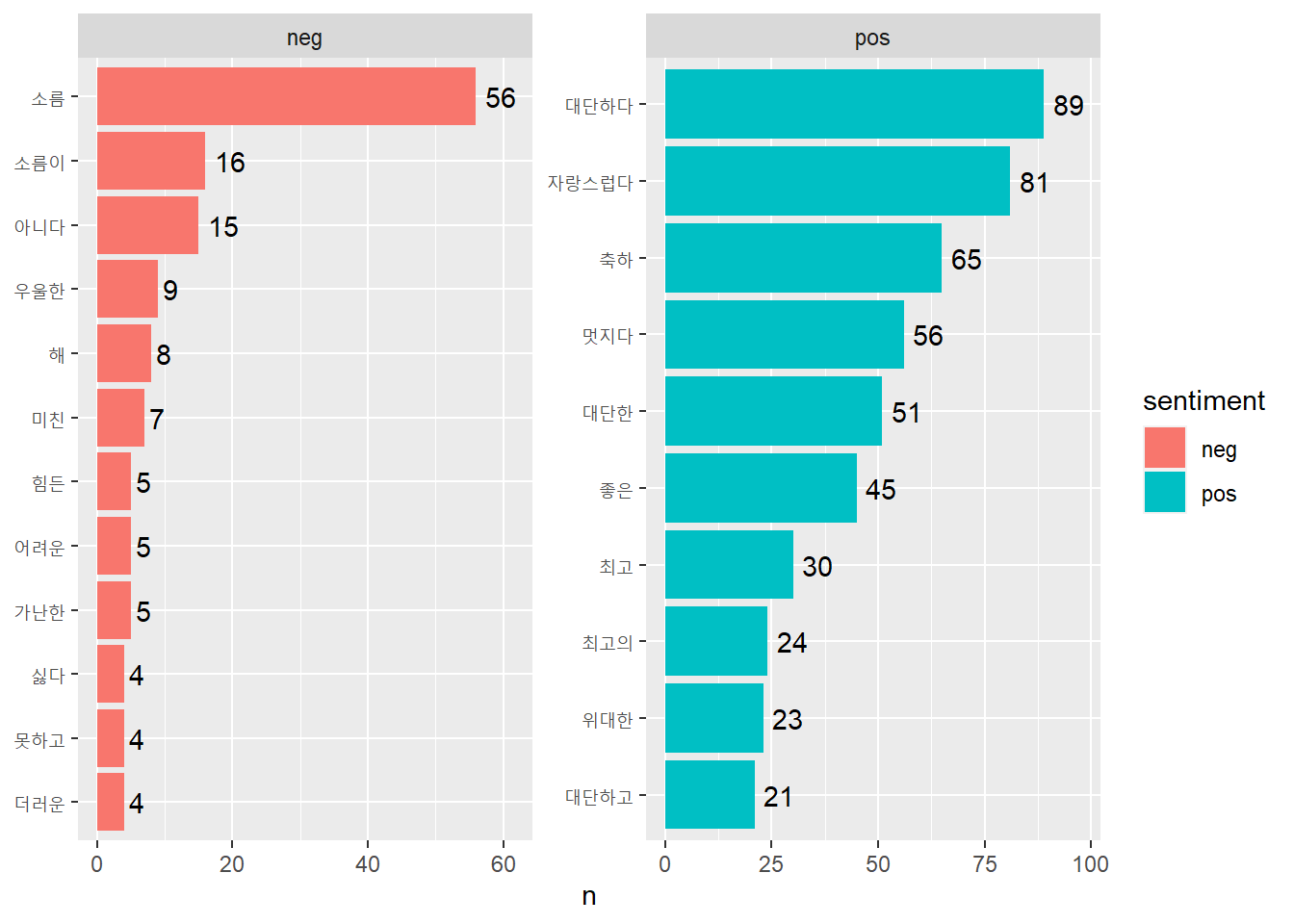
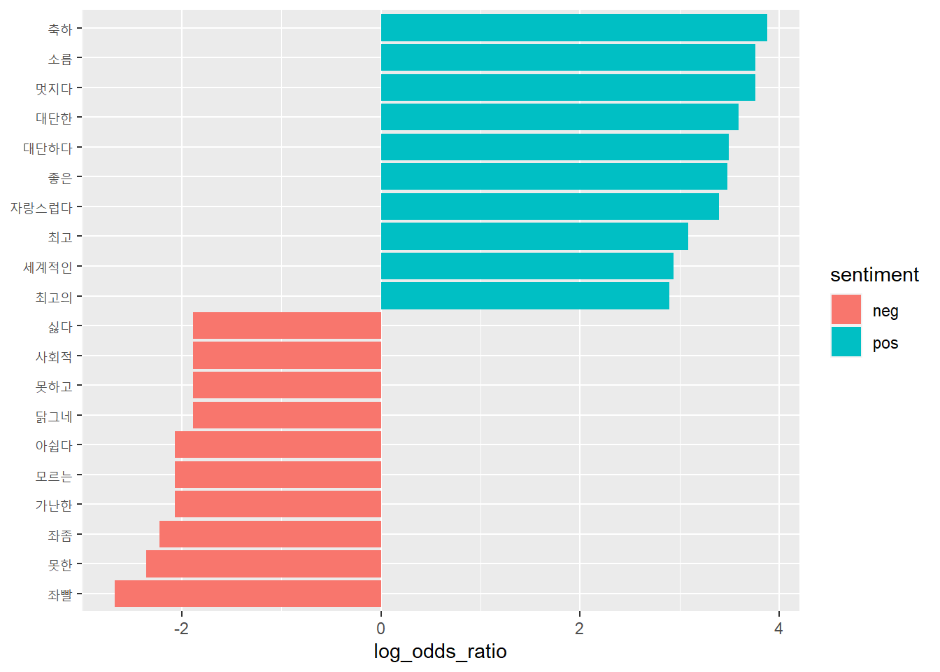
# 감정 범주별 주요 단어 살펴보기
# 1. 두 글자 이상 한글 단어만 남기고 단어 빈도 구하기
# 토큰화 및 전처리
new_comment <- new_score_comment %>%
  unnest_tokens(input = reply,
                output = word,
                token = "words",
                drop = F) %>%
  filter(str_detect(word, "[가-힣]") &
           str_count(word) >= 2)

# 감정 및 단어별 빈도 구하기
new_frequency_word <- new_comment %>%
  count(sentiment, word, sort = T)

# 2. 로그 오즈비 구하기
# Wide form으로 변환
new_comment_wide <- new_frequency_word %>%
  filter(sentiment != "neu") %>%
  pivot_wider(names_from = sentiment,
              values_from = n,
              values_fill = list(n = 0))

# 로그 오즈비 구하기
new_comment_wide <- new_comment_wide %>%
  mutate(log_odds_ratio = log(((pos + 1) / (sum(pos + 1))) /
                                ((neg + 1) / (sum(neg + 1)))))

# 3. 로그 오즈비가 큰 단어로 막대 그래프 만들기
new_top10 <- new_comment_wide %>%
  group_by(sentiment = ifelse(log_odds_ratio > 0, "pos", "neg")) %>%
  slice_max(abs(log_odds_ratio), n = 10, with_ties = F)

ggplot(new_top10, aes(x = reorder(word, log_odds_ratio),
                      y = log_odds_ratio,
                      fill = sentiment)) +
  geom_col() +
  coord_flip() +
  labs(x = NULL) 

# 4. 주요 단어가 사용된 댓글 살펴보기
# 긍정 댓글 원문
new_score_comment %>%
  filter(sentiment == "pos" & str_detect(reply, "축하")) %>%
  select(reply)

# A tibble: 189 × 1
   reply                                                                        
   <chr>                                                                        
 1 정말 우리 집에 좋은 일이 생겨 기쁘고 행복한 것처럼!! 나의 일인 양 행복합니다…
 2 와 너무 기쁘다! 이 시국에 정말 내 일같이 기쁘고 감사하다!!! 축하드려요 진심… 
 3 우리나라의 영화감독분들 그리고 앞으로 그 꿈을 그리는 분들에게 큰 영감을 주시…
 4 아카데미나 다른 상이나 지들만의 잔치지~ 난 대한민국에서 받는 상이 제일 가치 …
 5 정부에 빨대 꼽은 정치시민단체 기생충들이 득실거리는 떼한민국애서 훌륭한 영화…
 6 대단해요 나는 안봤는데 그렇게 잘 만들어 한국인의 기백을 세계에 알리는 큰 일… 
 7 나한테 돌아오는게 하나도 없는데 왜이렇게 자랑스럽지?ㅎㅎㅎ 축하 합니다~작품… 
 8 한국영화 100년사에 한횟을 긋네요. 정말 축하 합니다                           
 9 와 대단하다 진짜 축하드려요!!! 대박 진짜                                     
10 각본상, 국제 영화상 수상 축하. 편집상은 꽝남.                                
# ℹ 179 more rows

new_score_comment %>%
  filter(sentiment == "pos" & str_detect(reply, "소름")) %>%
  select(reply)

# A tibble: 77 × 1
   reply                                                                        
   <chr>                                                                        
 1 생중계 보며 봉준호 할 때 소름이~~~!! ㅠㅠ 수상소감들으며 함께 가슴이 벅차네… 
 2 와 보다가 소름 짝 수고들하셨어요                                             
 3 대단하다!! 봉준호 이름 나오자마자 소름                                       
 4 와우 브라보~ 키아누리브스의 봉준호, 순간 소름이.. 멋지십니다.                
 5 소름 돋네요. 축하합니다                                                      
 6 소름.... 기생충 각본집 산거 다시한번 잘했다는 생각이ㅠㅠㅠ 축하해요!!!!!!    
 7 봉준호 아저씨 우리나라 자랑입니다 헐리웃 배우들과 화면에 같이 비춰지는게 아… 
 8 추카해요. 봉준호하는데 막 완전 소름 돋았어요.                                
 9 소름돋아서 닭살돋고.. 그냥 막 감동이라 눈물이 나려했어요.. 대단하고 자랑스럽…
10 한국 영화 최초 아카데미상 수상, 92년 역사의 국제 장편 영화상과 최우수작품상 …
# ℹ 67 more rows

# 부정 댓글 원문
new_score_comment %>%
  filter(sentiment == "neg" & str_detect(reply, "좌빨")) %>%
  select(reply)

# A tibble: 34 × 1
   reply                                                                        
   <chr>                                                                        
 1 자칭 보수들은 분노의 타이핑중 ㅋㅋㅋㅋㅋㅋ전세계를 좌빨로 몰수는 없고 자존심…
 2 자칭보수 왈 : 미국에 로비했다 ㅋㅋ좌빨영화가 상받을리 없다 ㅋㅋㅋㅋㅋㅋㅋ 본…
 3 좌빨 봉준호 영화는 쳐다도 안본다 ㅋㅋㅋㅋㅋㅋㅋㅋㅋㅋㅋ                      
 4 봉준호 그렇게 미국 싫어하는데 상은 쳐 받으러 가는 좌빨 수준ㅋㅋㅋ            
 5 좌빨 기생충들은 댓글도 달지마라 미국 영화제 수상이 니들하고 뭔상관인데.      
 6 얘들은 왜 인정을 안하냐? ㅋㅋ 니들 이미 변호인 찍을대 부터 송강호 욕해대고 … 
 7 넷상 보수들 만큼 이중적인 새1끼들 없음. 봉준호 송강호 보고 종북좌빨 홍어드립…
 8 우선 축하합니다.그리고 다음에는 조씨가족을 모델로한 뻔뻔하고 거짓말을 밥 먹… 
 9 Korea 대단합니다 김연아 방탄 봉준호 스포츠 음악 영화 못하는게 없어요 좌빨 감…
10 좌빨 감독이라고 블랙리스트에 올랐던 사람을 세계인이 인정해주네. 방구석에 앉… 
# ℹ 24 more rows

new_score_comment %>%
  filter(sentiment == "neg" & str_detect(reply, "못한")) %>%
  select(reply)

# A tibble: 7 × 1
  reply                                                                         
  <chr>                                                                         
1 한번도경험하지. 못한 조국가족사기단기생충. 개봉박두                           
2 여기서 정치얘기하는 건 학창시절 공부 못한 거 인증하는 꼴... 주제좀 벗어나지 … 
3 이 기사를 반문으로 먹고 사는 자유왜국당과, mb아바타 간철수 댓글알바들이 매우 …
4 한국미국일본 vs 주적북한,중국러시아 이 구도인 현 시대 상황 속에서, 미국 일본… 
5 친일수꼴 들과 자한당넘들이 나라에 경사만 있으면 엄청 싫어합니다, 맨날 사고만 …
6 각본상,국제상,감독상 ...어디서 듣도보도 못한 아차상 같은 쩌리처리용 상 아닌가…
7 난 밥을 먹고 기생충은 오스카를 먹다, 기생충은 대한민국의 국격을 높였는데 난 … 

# 5. 분석 결과 비교하기
# 수정한 감정 사전 활용
new_top10 %>%
  select(-pos, -neg) %>%
  arrange(-log_odds_ratio)

# A tibble: 20 × 3
# Groups:   sentiment [2]
   word       log_odds_ratio sentiment
   <chr>               <dbl> <chr>    
 1 축하                 3.88 pos      
 2 멋지다               3.76 pos      
 3 소름                 3.76 pos      
 4 대단한               3.59 pos      
 5 대단하다             3.49 pos      
 6 좋은                 3.48 pos      
 7 자랑스럽다           3.40 pos      
 8 최고                 3.09 pos      
 9 세계적인             2.94 pos      
10 최고의               2.90 pos      
11 닭그네              -1.89 neg      
12 못하고              -1.89 neg      
13 사회적              -1.89 neg      
14 싫다                -1.89 neg      
15 가난한              -2.07 neg      
16 모르는              -2.07 neg      
17 아쉽다              -2.07 neg      
18 좌좀                -2.22 neg      
19 못한                -2.36 neg      
20 좌빨                -2.68 neg      

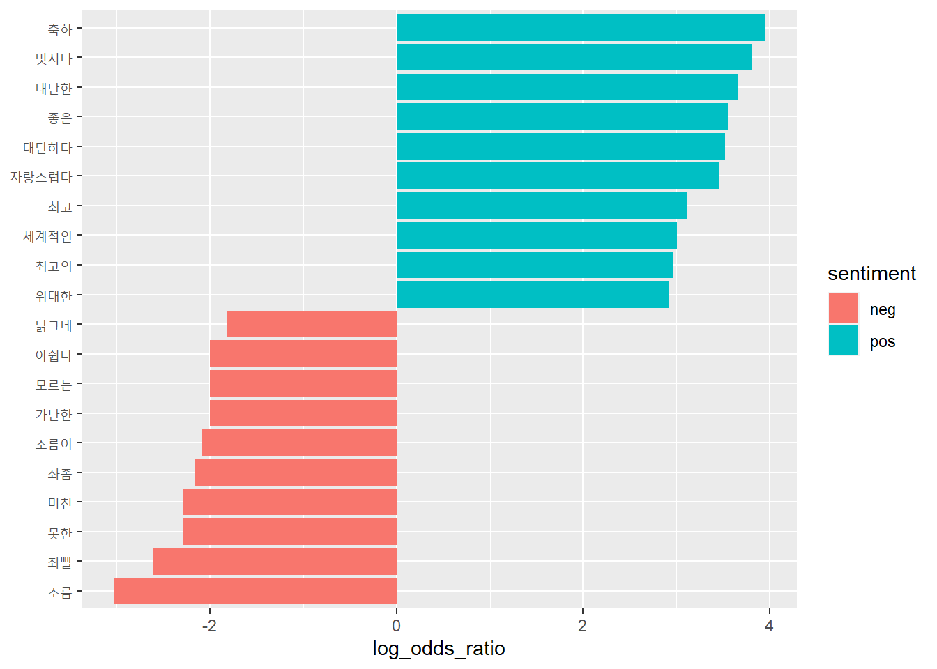
# 원본 감정 사전 활용
top10 %>%
  select(-pos, -neg) %>%
  arrange(-log_odds_ratio)

# A tibble: 20 × 3
# Groups:   sentiment [2]
   word       log_odds_ratio sentiment
   <chr>               <dbl> <chr>    
 1 축하                 3.95 pos      
 2 멋지다               3.81 pos      
 3 대단한               3.66 pos      
 4 좋은                 3.55 pos      
 5 대단하다             3.52 pos      
 6 자랑스럽다           3.46 pos      
 7 최고                 3.12 pos      
 8 세계적인             3.01 pos      
 9 최고의               2.97 pos      
10 위대한               2.92 pos      
11 닭그네              -1.82 neg      
12 가난한              -2.00 neg      
13 모르는              -2.00 neg      
14 아쉽다              -2.00 neg      
15 소름이              -2.08 neg      
16 좌좀                -2.16 neg      
17 못한                -2.29 neg      
18 미친                -2.29 neg      
19 좌빨                -2.61 neg      
20 소름                -3.03 neg      

# 수정 감정 사전 활용 시 "미친"이 목록에서 사라짐, 로그 오즈비가 10위 안에 들지 못할 정도로 낮아지기 때문
new_comment_wide %>%
  filter(word == "미친")

# A tibble: 1 × 4
  word    pos   neg log_odds_ratio
  <chr> <int> <int>          <dbl>
1 미친      7     0           1.80